In this project we quantitatively analyzed the behaviour of the output of the GPT-2 LLM and its dependence on the temperature parameter that is used in the final Sofmax layer of probabilities. It has been noticed that as temperature decreases towards absolute zero, the text output of neural networks, such as GPT-3.5 and GPT-4, tends to become completely deterministic and uncreative, while as temperature increases arbitrarily the sentences that are output by the LLM become chaotic and nonsensical. Therefore, the question of the existence of a critical temperature at which LLMs exhibit an abrupt transition between these two types of behaviour arises; as well as the question of this potential critical temperature being the hallmark of a phase transition-like process in LLMs. The hypothesis of this project is that there is a critical temperature at which some set of quantitative parameters associated to LLMs changes abruptly, or shows some noticeable qualitative change. The main goal of this project is therefore to identify an appropriate quantitative parameter associatede to the output of an LLM, and see how it behaves at increasingly low temperatures. In order to achieve this, the GPT-2 neural net trained on WebText data was used, which is available in the Wolfram neural net repository. With this neural net, the correlations between tokens at different positions of ouput strings was measured, using the statistical tools of the Wolfram Language, so as to see at which temperature these correlations freeze out to 1. Also, the mean squared displacement of the embedding vectors of each successive token was measured, so as to determine if random-walk stochastic behaviour is detected above the temperature that would be found in the previous approach. It was concluded that there is a non-zero finite critical temperature of the order of 0.1 where GPT-2 becomes completely deterministic, and loses all creativity. Also, the phase above this onset of determinism is not completely stochastic, which suggests that the phase above the critical temperature is not characterized by Markov-like random processes.
Introduction (basics of LLMs, and the meaning of temperature)
Introduction (basics of LLMs, and the meaning of temperature)
Text generation in GPT-2
Text generation in GPT-2
The rise of AI in the form of Large Language Models (LLMs) has now been mainstream since the release of the first publicly available version of Chat-GPT back in 2022. These LLMs are basically neural networks trained on very large amounts of data from the internet, in order to generate text in a way that is as similar as possible to natural language. The basic way that LLMs such as ChatGPT work is by taking in a sequence of text (in programming words, a string of text), and they associate it to a certain array of numbers that it can perform linear algebra operations upon. As Wolfram (2023) puts it, each individual set of operations is associated to a specific “neuron” of the neural net, which passes the resulting array of numbers to the following set of neurons, so they can perform more numerical operations of their own (this is why we call these systems neural nets or neural networks, since they are meant to mimic the behaviour of neurons in a human brain). The basic schematics of a neural network can be visualized in the following graph, retrieved from the work of Wolfram (2023):
Out[]=
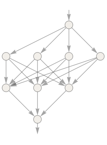
Once all the numerical operations are performed, the resulting array of numbers is associated back to a specific string of text, which corresponds to the word (or sub-word/sequence of characters) that the neural net concludes is the most likely to follow the text that it has been given. With this picture in mind, we can see that basically what ChatGPT does is produce one single word (or sub-word/sequence of characters) at a time, which is meant to follow a specific input of text in a (hopefully) coherent and cohesive way (Wolfram, 2023).
Now, the mechanism through which GPT associates words to arrays of numbers in the first place is the main point of interest of this project. Indeed, after all of its training, the neural net “learns” how to split up any string of text into sub-components, ore “tokens”, which correspond to a specific set (in the case of GPT-2 there are in the order of 50,000 tokens) of words and subwords/sequences of characters. For example, the text: “Hello world!” might be broken up in the sub-components: “He”, “llo”, “ “, “world”, “!” . Each token is associated to a certain embedding vector, which corresponds to a 768-dimensional (in the case of GPT-2) vector, and is associated specifically to the token based on its characters and position relative to the rest of the tokens in the input text. Embedding vectors are said to reside in “meaning space”, which is just a way of saying that these vectors capture the context and meaning of each token based on the sentence they are placed into.The main process of embedding is performed in the first layer of the neural net (the embedding layer) and can be visualized as follows:
Now, the mechanism through which GPT associates words to arrays of numbers in the first place is the main point of interest of this project. Indeed, after all of its training, the neural net “learns” how to split up any string of text into sub-components, ore “tokens”, which correspond to a specific set (in the case of GPT-2 there are in the order of 50,000 tokens) of words and subwords/sequences of characters. For example, the text: “Hello world!” might be broken up in the sub-components: “He”, “llo”, “ “, “world”, “!” . Each token is associated to a certain embedding vector, which corresponds to a 768-dimensional (in the case of GPT-2) vector, and is associated specifically to the token based on its characters and position relative to the rest of the tokens in the input text. Embedding vectors are said to reside in “meaning space”, which is just a way of saying that these vectors capture the context and meaning of each token based on the sentence they are placed into.The main process of embedding is performed in the first layer of the neural net (the embedding layer) and can be visualized as follows:
Out[]=
NetGraph


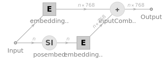

Indeed, the input string is taken in, and decomposed into n tokens (where n is an integer that indicates the number of tokens that the input consists of). Each token is associated to a specific natural number that identifies it from the rest of the tokens (for example the label for the token “A” is the number 50,225). Once this is done, the list of n tokens is fed into two different embedding layers, where each one of them associates to each of the n natural numbers that it receives a specific embedding vector (list of 768 real numbers). Then, these two - dimensional arrays are combined to give a final - dimensional array. This is just the first embedding phase, however, for now comes the “real” main section of the whole process. Once the list of embedding vectors is produced, it is passed through a sequence of “attention layers” (Wolfram, 2023). The first attention layer looks, schematically, like this:
n768
n768
In[]:=
NetFlatten[NetExtract[NetModel["GPT2 Transformer Trained on WebText Data"],{"decoder","1"}]]
Out[]=
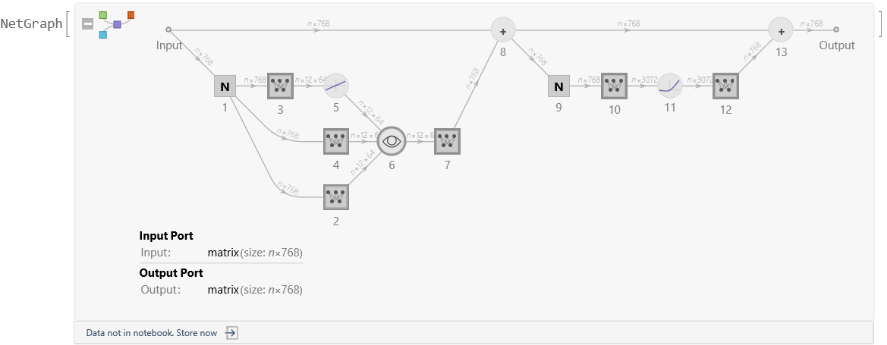
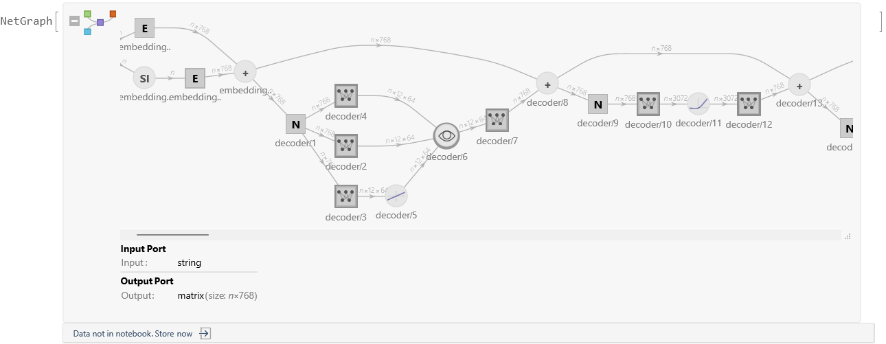
In each of these nodes, specific linear algebra operations are performed onto the initial - dimensional array. The weights of the linear operations in each node have been tuned specifically during the training process of the neural net (Wolfram, 2023). They are called “attention layers” because the operations performed are a way of, technically, “looking back” on the structure of the whole string, so that the final sequence embedding arrays produced will take into account the whole structure of the text, and not just the final tokens that precede the one that the neural net is expected to generate (Wolfram, 2023). In the case of GPT-2, there are exactly twelve of these attention layers in the whole body of the neural network:
n768
In[]:=
NetFlatten[NetModel["GPT2 Transformer Trained on WebText Data"]]
Out[]=
For example, here’s what the resulting embedding array for the text “Hello, world! I am here and am very happy to be!” looks like:
Out[]=

Each row is a different embedding vector for a different token, and we can see that, in this case, the input text was decomposed into 14 constituent tokens. Thus, the whole operation of creating a single token of text from a given input can be summarised as the mapping between a first array of embedding vectors and a final array of embedding vectors:
Out[]=
| ||
↓ | ||
|


The way GPT translates the final embedding vector into a token (presumably the likeliest piece of text that follows the text that was input in the first place) is the topic of the next subsection.
Softmax layer and temperature parameter
Softmax layer and temperature parameter
The final embedding array shown in the previous section is meant to represent “the essence” of the sentence that was given to the LLM. From this essential collection of 768-dimensional vectors, the LLM will have to make the decision of which token follows the original text. The way GPT-2 is constructed makes it take only the last embedding vector as a representative of the whole sentence, and from this embedding vector it generates a sequence of probabilities; one for each token that the transformer has access to, and they correspond, clearly, to the probability of each of these tokens to follow the original text. Then, based on these probabilities the LLM chooses the following token, and finally generates the resulting text.Now, backing up a bit, once the LLM has extracted the last embedding vector from the embedding array, it uses a final linear layer (which is just a layer that performs a final set of linear-algebra operations on the vector)to go from a list of 768 real numbers to a list of 50,257 negative numbers. Each of these numbers is the “weight” that each possible token has regarding how likely it is to be the token that the LLM will choose. This list of numbers is the “normalized” through the final SoftMax layer, which takes each of these weights and converts them into an actual probability value (a number between 0 and 1), such that all probabilities add up to 1, as a proper probability distribution should (Wolfram Language, 2016). The specific formula that converts from the list of weights into a probability vector is through the Maxwell-Boltzmann canonical distribution formula:
(,,…,)
E
1
E
2
E
50257
(,,…,)
p
1
p
2
p
50257
p
j
β
E
j
e
Z
50257
∑
j1
β
E
j
e
(
1
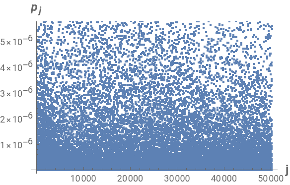
)The factor β that is included in the exponent is the inverse temperature factor; a concept borrowed from statistical mechanics which corresponds to the multiplicative inverse of a positive parameter that is associated to the “temperature” of a system: . This temperature parameter influences the shape of the distribution that the LLM uses to choose the resulting token; making it more uniform as the temperature becomes higher (thus making β smaller), and therefore making the choices of the LLM more random and “creative”.
β, T>0
1
T
Out[]=
,
T = 1 |
T = 0.01 |
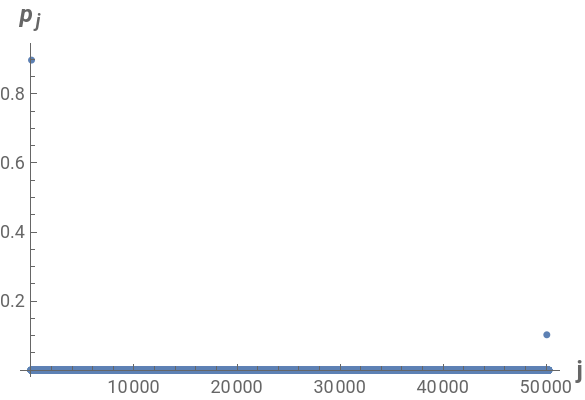
As we can see, high temperatures result in more spread-out probabilities for each of the labeled 50,257 tokens that GPT-2 supports, while smaller temperatures result in more localized probabilities around specific tokens, leading to less creative and more deterministic results. It is expected, therefore, that at very high temperatures the LLM will behave no different from a regular random word generator, losing all coherence; while at very low temperatures it will behave very deterministically and with no creativity. Indeed, here is an example of the difference of behaviour:
In[]:=
generateTextInefficient["I am very happy to be",40,0.]
Out[]=
I am very happy to be here. I am very happy to be here. I am very happy to be here. I am very happy to be here. I am very happy to be here. I am very happy to be
In[]:=
generateTextInefficient["I am very happy to be",40,0.45]
Out[]=
I am very happy to be of service to you.We have been working together since 2010. We have had a number of improvements and we are very pleased with the results.We have been working together since
Having all of the previous facts in mind, the main goal of this project is to measure quantitatively when the GPT-2 LLM makes the actual change from being a deterministic, no-fun text generator at “low temperatures”. More precisely: is there some quantitative measure that helps us determine a critical temperature at which the LLM “goes bonkers”? (Stephen Wolfram, personal comunication). In order to answer this question, we will borrow concepts and methods from thermodynamics and statistical mechanics, since these disciplines deal with the study of phase transitions in the material world, which would be the closest concept that we can apply to what we actually expect to happen to an LLM at some critical temperature: it should go from one phase of “being bonkers” to a different phase of “being completely deterministic”.
Main results
Main results
1.-Calculation of entropy for various inputs
1.-Calculation of entropy for various inputs
One of the first direct links that can be drawn between an LLM, as was exposed in the previous section, is its entropy, given by the following formula, due to Shannon (Pathria & Beale, 2011):
The information entropy of a system is a measure of the disorder, or unpredictability, of the outcome of a measurement of the system itself. The sum in eq. (2) is taken over all possible “microstates” of the system. In the case of GPT-2, the system can be thought of as the collection of all possible tokens that can follow a certain input string (with each token representing a possible microstate), with their corresponding probabilities the values assigned to them through the Softmax layer. Of course, the entropy itself would depend on the values of the weights assigned to each token in the layer before the Softmax, and therefore on the exact input (giving “Hello world!” as input would result in a different distribution that “Hello!”, and therefore they would be assigned different entropies).
With the previous information in mind, let’s calculate the entropy for a random sample of different inputs, and plot their behaviour with respect to temperature. In order to do that, a large sample of random sentences from three books will be used as a big enough “universe” of inputs from which to choose prompts for GPT-2.
With the previous information in mind, let’s calculate the entropy for a random sample of different inputs, and plot their behaviour with respect to temperature. In order to do that, a large sample of random sentences from three books will be used as a big enough “universe” of inputs from which to choose prompts for GPT-2.
As it can be seen, the behaviour of the entropies for all these different show the same qualitative behaviour. Besides from the obvious characteristics of Shannon entropy (being an increasing function of temperature, and tending towards zero as the temperature also goes to zero), all entropy curves seem to depart from being practically zero at around the same range of temperatures:
2.- Correlations between tokens at different positions in output text
2.- Correlations between tokens at different positions in output text
In the field of physics, when a large quantum system undergoes a second-order phase transition, the different components tend to be completely correlated to one another. Said another way, the Pearson correlation coefficient:
However, if we change only slightly the input text, then of course the resulting output will most certainly be different at every iteration that is performed.
3.- Analysis of stochastic behaviour of embedding vectors
3.- Analysis of stochastic behaviour of embedding vectors
In our case, for a string of large tokens, where each new token added to the string by GPT-2 corresponds to a new step in the random process, we don’t know the actual probability distribution for each token, since this depends on the weights associated to each token itself, which in turn depends on the internal architercture and weights of the neural network, which goes beyond the scope of this works. Therefore, we should take, for fixed temperature, a large statistical sample of the generation of long tokens, and take the average of the quadratic deviation of the resulting embedding vector at each step over said sample. The text over we will iterate will be the very same as in the last section: “The first letters of the alphabet are:”
Results
Results
Concluding remarks
Concluding remarks
Keywords
Keywords
◼
LLM
◼
GPT-2
◼
Embedding vector
◼
Entropy
◼
Correlation coefficient
◼
Phase transition
◼
Critical temperature
Acknowledgment
Acknowledgment
I’d like to thank my mentor, Christian Pasquel, for his invaluable advice and help in the creation of this Summer School Project. His insight into what approach to follow at the various steps of the project was of tremendous help. I’d also like to thank the great help of the Summer School’s TAs, who came to my aid when I found myself stuck in some coding conundrum, or when I needed to make my code more efficient; specifically, Mark Greenberg, Daniel Sánchez, Jofre Espiguel, Christopher Wolfram, and Robert Nachbar helped me a great deal to reach the conclusion of this project.
References
References
◼
Wolfram Language (2016), SoftmaxLayer, Wolfram Language & System Documentation Center. Retrieved from:https://reference.wolfram.com/language/ref/SoftmaxLayer.html
◼
Wolfram Research (2021), NetUnfold, Wolfram Language function, https://reference.wolfram.com/language/ref/NetUnfold.html.
◼
Pathria, R.K. and Beale, P.D. (2011). The canonical ensemble. In Pathria, R.K. and Beale, P.D. (Eds.), Statistical Mechanics (Third edition, pp. 50-54). Elsevier.
◼
Kardar, M. (2007). Statistical Physics of Fields. (First edition). Cambridge University Press
◼
Wolfram Research (2022), GPT-2 transformer trained on WebText data. Retrieved from: https://resources.wolframcloud.com/NeuralNetRepository/resources/GPT2-Transformer-Trained-on-WebText-Data/
CITE THIS NOTEBOOK
CITE THIS NOTEBOOK
Study of the possibility of phase transitions in LLMs
by Sebastián Bahamondes
Wolfram Community, STAFF PICKS, July 12, 2023
https://community.wolfram.com/groups/-/m/t/2958851
by Sebastián Bahamondes
Wolfram Community, STAFF PICKS, July 12, 2023
https://community.wolfram.com/groups/-/m/t/2958851