Introduction to Variational Quantum Algorithms
Introduction to Variational Quantum Algorithms
Introduction
Introduction
Quantum computing has long been envisioned as a transformative technology, with the potential to tackle problems that are intractable for classical computers. Quantum algorithms promise exponential speedups in areas such as number factorization, quantum system simulation, and solving linear systems of equations.
The introduction of cloud-based quantum computers in 2016 provided public access to real quantum hardware. However, due to noise and the limited number of qubits, running large-scale quantum algorithms remained impractical. This led to growing interest in what could be achieved with these early devices, commonly referred to as Noisy Intermediate-Scale Quantum (NISQ) computers. Today’s state-of-the-art NISQ devices contain up to 1000 qubits, with only two quantum processors having over 1,000 qubits, making it possible to surpass classical supercomputers in specific, carefully designed computational tasks—a milestone known as quantum supremacy.
Variational Quantum Algorithms (VQAs) have emerged as the leading approach for using the power of NISQ devices. Given the constraints of current quantum hardware, VQAs employ a hybrid quantum-classical optimization framework. They utilize parameterized quantum circuits executed on a quantum computer, while classical optimizers adjust the parameters to minimize a given cost function. This strategy mirrors machine-learning techniques, such as neural networks, which rely on optimization-based learning methods.
Applications
Applications
VQAs have been explored for a wide range of applications, spanning nearly all areas initially envisioned for quantum computing. As illustrated in the following image, VQAs are applied across various domains, including error correction, machine learning, combinatorial optimization, ground-state estimation, and mathematical problem-solving.
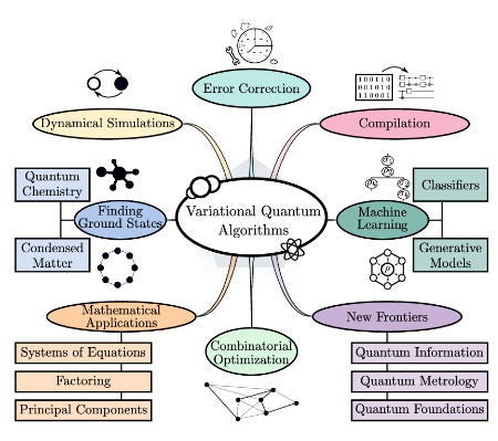
Cerezo, M., Arrasmith, A., Babbush, R. et al. Variational quantum algorithms. Nat Rev Phys 3, 625–644 (2021)
While they hold promise for achieving near-term quantum advantage, significant challenges remain, including issues related to trainability, accuracy, and efficiency. Addressing these challenges is crucial for the continued advancement of VQAs and their practical implementation in solving real-world problems.
In simple terms, Variational Quantum Algorithms (VQAs) are one of the most popular approaches for running quantum algorithms on today’s early-stage quantum computers. You can think of VQAs like “putting the carriage before the horses”, we know what problem we want to solve, but we don’t yet know the exact quantum circuit to do it. Instead of designing the circuit manually, VQAs use classical optimization techniques to “learn” the best circuit for the task.
Pipeline
Pipeline
The core components of this algorithms include a parameterized quantum circuit, known as the ansatz, which is used to represent possible solutions. This ansatz is evaluated through a cost function that encodes the problem we are trying to solve. Finally, a training procedure, primarily driven by a classical optimizer, adjusts the parameters of the ansatz to improve the solution iteratively.
Out[]=
This process is best illustrated in the Hybrid Loop shown in the next image. The quantum computer runs the ansatz, the results are evaluated through the cost function, and the classical optimizer processes this information to update the parameters for the next iteration.
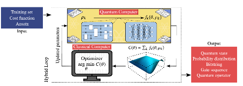
Cerezo, M., Arrasmith, A., Babbush, R. et al. Variational quantum algorithms. Nat Rev Phys 3, 625–644 (2021)
Now, rather than just describing it, let’s dive into parametrized circuits!
Load Wolfram Quantum Framework
Load Wolfram Quantum Framework
First, we need to load the Wolfram Quantum Framework. Below is the command to install it, and if you already have it, simply load it:
In[]:=
PacletInstall["https://wolfr.am/DevWQCF",ForceVersionInstall->True]
Out[]=
PacletObject
In[]:=
<<Wolfram`QuantumFramework`
Parametrized Quantum Circuits
Parametrized Quantum Circuits
Variational Quantum Algorithms rely on Parameterized Quantum Circuits, a fancy term for quantum circuits that include gates with adjustable parameters. This algorithms work by exploring and comparing variational states that depends on a set of parameters.
|ϕ(θ)〉
{θ}
n
You can build this variational states using a fixed initial state as and a parametrized or variational quantum circuit :
|0〉
V(θ)
|ϕ(θ)〉=V(θ)|0〉
Think of it this way: some quantum gates, like rotation gates, depend on a variable angle, while others, like Hadamard (H) gates or CNOT gates, have fixed operations with no adjustable parameters.
We aim to train these variational quantum circuits using a classical optimizer that fine-tune these parameters, in conjunction with a cost function that reflects the objective of our optimization.
Since the Wolfram Quantum Framework operates symbolically, defining parameterized quantum circuits is a natural process. This allows us to work with symbolic parameters instead of fixed numerical values, making it easier to optimize and analyze circuits.
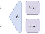
Wolfram Quantum Framework supports "free parameters" in their quantum circuits, you only need to specify this tunable parameters by using the "Parameters" option:
vqc=QuantumCircuitOperator[{"00","RX"[θ1]{1},"RY"[θ2]{2}},"Parameters"{θ1,θ2}];
In[]:=
vqc["Diagram"]
Out[]=
The parameters defined for a Wolfram Quantum Framework Operator are heritable, so you do not need to redefine it in later steps. For example we can calculate the resultant state from our defined variational circuit:
|ϕ(θ)〉
In[]:=
vqs=vqc[]
Out[]=
QuantumState
We can verify that the "Parameters" option values:
In[]:=
vqs["Parameters"]
Out[]=
{θ1,θ2}
This option simplifies the repeated execution of the circuit by using the symbolic computation capabilities provided by the Wolfram Quantum Framework:
In[]:=
vqc["Formula"]
Out[]=
CosCos|00〉+CosSin|01〉-CosSin|10〉-SinSin|11〉
θ1
2
θ2
2
θ1
2
θ2
2
θ2
2
θ1
2
θ1
2
θ2
2
Replace θ1 value as follows:
In[]:=
vqc[θ10]["Formula"]
Out[]=
Cos|00〉+Sin|01〉
θ2
2
θ2
2
As mentioned earlier, you can use the parameters at any stage of your algorithm, as they are carried through each step:
In[]:=
vqs["Formula"]
Out[]=
CosCos|00〉+CosSin|01〉-CosSin|10〉-SinSin|11〉
θ1
2
θ2
2
θ1
2
θ2
2
θ2
2
θ1
2
θ1
2
θ2
2
In[]:=
vqs[θ20,θ10]["Formula"]
Out[]=
|00〉
You can directly replace the values for each parameter following the same order you defined them:
In[]:=
vqs[0,0]["Formula"]
Out[]=
|00〉
In[]:=
vqs[a,b]["Formula"]
Ansatz circuits
Ansatz circuits
Initial State Preparation
Initial State Preparation
If you have an educated guess or an existing optimal solution, using it as the reference state can help the variational algorithm converge faster.
The simplest reference state is the default state, where we initialize an n-qubit quantum circuit in the all-zero state:
For this default state, our unitary operator is simply the identity operator. Due to its simplicity, this default state is widely used as a reference state in many applications.
If we want to start with a more complex reference state that involves superposition and entanglement, we can prepare a state such as:
Which is also called a Bell State:
Ansatz Circuits
Ansatz Circuits
In physics and mathematics, the German word “Ansatz” refers to an educated guess for solving a problem. You may have done this before—trying out a potential solution based on intuition or prior knowledge. However, an ansatz is not just any guess; it must be well-informed.
In Variational Quantum Algorithms (VQAs), what we are guessing is the quantum circuit that will solve our problem. This is why we refer to this circuit simply as the ansatz
Generate a collection of parametrized states:
How Do We Choose an Ansatz?
◼
Problem-Inspired Ansatz
◼
If we have prior knowledge about the problem, we can use physical intuition or mathematical insights to design a circuit tailored to the task. This approach typically leads to more efficient circuits with fewer parameters, making optimization easier. These are usually referred to generally as Hardware-Efficient ansatz.
◼
Problem-Agnostic Ansatz
◼
If we lack detailed knowledge about the problem, we can use a more general universal ansatz that does not rely on problem-specific intuition. These ansatze are more expressive, meaning they can represent a wide range of solutions. However, they also tend to be larger, with more gates and parameters, making the optimization process significantly harder.
If we consider this simple ansatz, consisting of a pair of rotations and a CNOT gate, we can evaluate it and examine the states that can be generated:
As we observe, the possible states generated by this ansatz are limited to those determined by the sine and cosine functions. Therefore, even with an excellent optimizer, there will be certain values that this ansatz will never be able to reach:
How good is an ansatz?
◼
Expressibility
◼
This measures the range of functions that the quantum circuit can represent. Higher expressibility is generally linked to more entanglement and a greater number of parameters. The more expressive an ansatz is, the more problems it can potentially solve.
◼
Trainability
◼
This refers to how easy it is to find the right parameters for the circuit. Larger, highly expressive circuits are harder to optimize because the optimizer must explore a vast parameter space. The difficulty of training also depends on the cost function and the classical optimizer used.
There is a natural trade-off between expressibility and trainability. Highly expressive circuits are powerful but harder to train, while simpler circuits may be easier to optimize but might not capture the necessary complexity of the problem.
The goal is to find an ansatz in the “sweet spot”—one that is expressive enough to solve the problem but still trainable within a reasonable amount of time.
Now, let’s explore this concept further with an exercise!
◼
Exercise 1:
Express the collection of parametrized states generated by the following ansatz:
Step by step:
◼
Exercise 2:
Express the collection of parametrized states generated by the following ansatz:
Following the same steps:
We can verify that the second ansatz has more expressibility by the simple fact that:
The first ansatz is a specific case of the second ansatz:
What happens if we have no idea about the problem solution?
Layered gate architectures, where the ansatz is repeated multiple times, have been shown to offer a good balance between expressibility and relatively low circuit depth, making them effective for tackling a broad range of problems.
If the problem we are trying to solve doesn’t require a large number of parameters, a good option might be to use an ansatz called the Basic Entangler. This ansatz is often favored for its simplicity and efficiency in cases where the problem doesn’t demand an overly complex parameterized quantum circuit. This layers consist of one-parameter single-qubit rotations on each qubit, followed by a closed chain or ring of CNOT gates.
Cost functions and optimization
Cost functions and optimization
Once we have the ansatz circuit, the next step is to determine the parameters that we need to input in order to perform the task at hand. So, how do we do this? This is accomplished by defining a cost function, which measures how close the output of the circuit is to the desired result.
The goal most of the time is to minimize a cost function. This is the essence of many variational algorithms, we adjust the parameters iteratively to find the minimum value of the cost function, which indicates the best solution, even when the exact answer is not known in advance.
In variational quantum algorithms, we usually define the cost function as the expectation value of a given observable ℋ:
Let’s test this simple example of a Hamiltonian conformed by Pauli operators in two qubits.:
After constructing the ansatz, we compute it to obtain the resultant quantum state, which we can represent as the “StateVector.” From here, we define the corresponding ket and bra states.
To build the cost function, we calculate the expectation value by applying the Hamiltonian H to the bra and ket states that we computed.
Since our result is symbolic, we can visualize how the cost function behaves across a range of values for the parameters.
This visualization gives us insight into the behavior of the function, showing us a spectrum of values. Among these, we can identify the minimal values.
To pinpoint the precise parameters that correspond to the minimum, we use the FindMinimum function. This will give us the exact pair of parameters that achieve the minimum value.
The result is logical: when θ1 is either π or −π, we consistently observe the minimum value of approximately −0.8-This is in line with our expectations, confirming that the optimization process is working correctly.