Fourier Series Approximation of a Triangular Wave Function
Authors: Housam Binous and Ahmed Bellagi
Fourier Series Approximation of a Triangular Wave Function
Authors: Housam Binous and Ahmed Bellagi
Authors: Housam Binous and Ahmed Bellagi
We show how one can find the approximate Fourier representation of a triangular wave function.
Triangular Wave Function
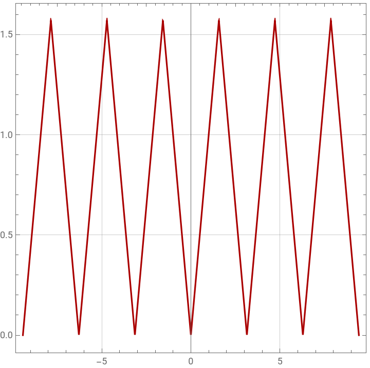
Plot of the function f(t) in red
Plot of the function f(t) in red
In[]:=
g[t_]:=If[t<0,0,If[t<Pi/2,t,If[Pi>t>Pi/2,Pi-t,0]]]
In[]:=
f[t_]:=If[t<Pi||t>Pi,g[t-Quotient[t,Pi]Pi],g[t]]
In[]:=
plt1=Plot[f[t],{t,-3Pi,3Pi},PlotStyleDarker@Red,FrameTrue,GridLinesAutomatic,AspectRatio1,ImageSizeMedium]
Out[]=
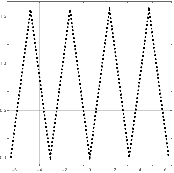
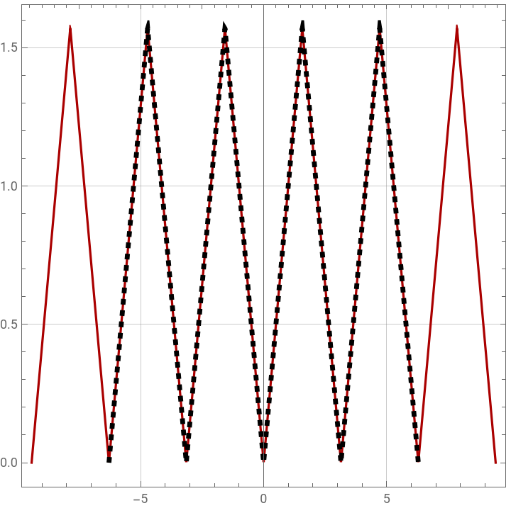
Generating the same plot (in dashed black) using the built-in command TriangleWave
In[]:=
plt1b=Plot[PiTriangleWave[{0,1/2},1/Pi(t-Pi/4)],{t,-2Pi,2Pi},PlotRangeAll,PlotStyle{Dashed,Black,Thickness[0.01]},FrameTrue,GridLinesAutomatic,AspectRatio1,ImageSizeMedium]
Out[]=
In[]:=
Show[plt1,plt1b]
Out[]=
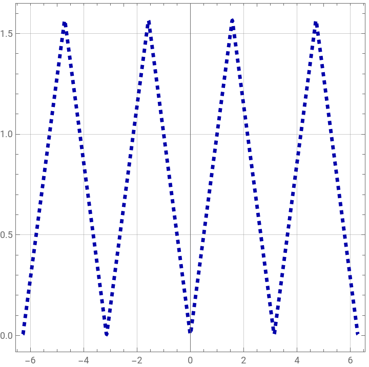
Plot of the Fourier series approximation of f(t) in dashed blue
In[]:=
LaunchKernels[]
Out[]=
{KernelObject[1,local],KernelObject[2,local]}
In[]:=
a=Parallelize@Table[NIntegrate[f[t]Cos[2iPit/Pi],{t,0,Pi},AccuracyGoal->4]/Pi,{i,1,50}]
Out[]=
{-0.31831,5.2672×,-0.0353678,-2.24407×,-0.0127324,1.20645×,-0.00649612,-4.00509×,-0.00392975,1.90695×,-0.00263066,-2.42755×,-0.00188349,4.55415×,-0.00141471,-1.64177×,-0.00110142,5.54332×,-0.000881745,1.35207×,-0.000721791,-1.5447×,-0.00060172,-2.4194×,-0.000509296,1.0548×,-0.000436639,-8.64277×,-0.00037849,-1.28177×,-0.000331228,2.69809×,-0.000292296,1.16528×,-0.000259845,6.72299×,-0.000232513,2.07254×,-0.000209277,1.10098×,-0.000189357,2.02552×,-0.000172152,-1.43258×,-0.00015719,-6.15932×,-0.000144097,1.27987×,-0.000132574,8.09713×}
-17
10
-16
10
-16
10
-17
10
-16
10
-16
10
-16
10
-16
10
-17
10
-16
10
-16
10
-17
10
-16
10
-17
10
-16
10
-18
10
-16
10
-17
10
-17
10
-16
10
-17
10
-16
10
-17
10
-17
10
-17
10
In[]:=
b=Parallelize@Table[NIntegrate[f[t]Sin[2iPit/Pi],{t,0,Pi},AccuracyGoal->4]/Pi,{i,1,50}]
Out[]=
{3.53395×,-3.53395×,-1.06018×,0.,1.85532×,1.76697×,8.83487×,-9.27662×,1.94367×,3.40143×,3.53395×,-7.64217×,1.81115×,5.76476×,-3.15847×,2.20872×,-1.94367×,1.78906×,-4.41744×,2.29707×,2.65046×,1.45775×,5.96354×,4.63831×,5.74267×,-2.87133×,4.74874×,-6.73659×,3.31308×,-8.06182×,1.87741×,-8.06182×,3.31308×,-7.17834×,-2.20872×,-6.07398×,-1.10436×,-4.74874×,-1.2148×,-3.75482×,-1.43567×,-2.65046×,-1.87741×,-1.87741×,-1.76697×,-1.2148×,-1.65654×,-7.73051×,-1.76697×,-3.31308×}
-17
10
-17
10
-16
10
-16
10
-17
10
-18
10
-17
10
-16
10
-16
10
-17
10
-16
10
-16
10
-16
10
-16
10
-18
10
-16
10
-16
10
-17
10
-16
10
-17
10
-16
10
-17
10
-17
10
-17
10
-17
10
-17
10
-17
10
-17
10
-17
10
-17
10
-17
10
-18
10
-17
10
-18
10
-17
10
-17
10
-17
10
-17
10
-17
10
-17
10
-17
10
-17
10
-17
10
-17
10
-17
10
-17
10
-18
10
-17
10
-18
10
In[]:=
b//Chop(*barrayhasonlynilelementsbecausef(t)isanevenfunction*)
Out[]=
{0,0,0,0,0,0,0,0,0,0,0,0,0,0,0,0,0,0,0,0,0,0,0,0,0,0,0,0,0,0,0,0,0,0,0,0,0,0,0,0,0,0,0,0,0,0,0,0,0,0}
In[]:=
a0=2/PiNIntegrate[f[t],{t,0,Pi},AccuracyGoal->4]
Out[]=
1.5708
In[]:=
plt2=Plot0.5a0+2(a[[i]]Cos[2iPix/Pi]+b[[i]]Sin[2iPix/Pi]),{x,-2Pi,2Pi},PlotRangeAll,PlotStyle{Dashed,Darker@Blue,Thickness[0.01]},FrameTrue,GridLinesAutomatic,AspectRatio1,ImageSizeMedium
50
∑
i=1
Out[]=
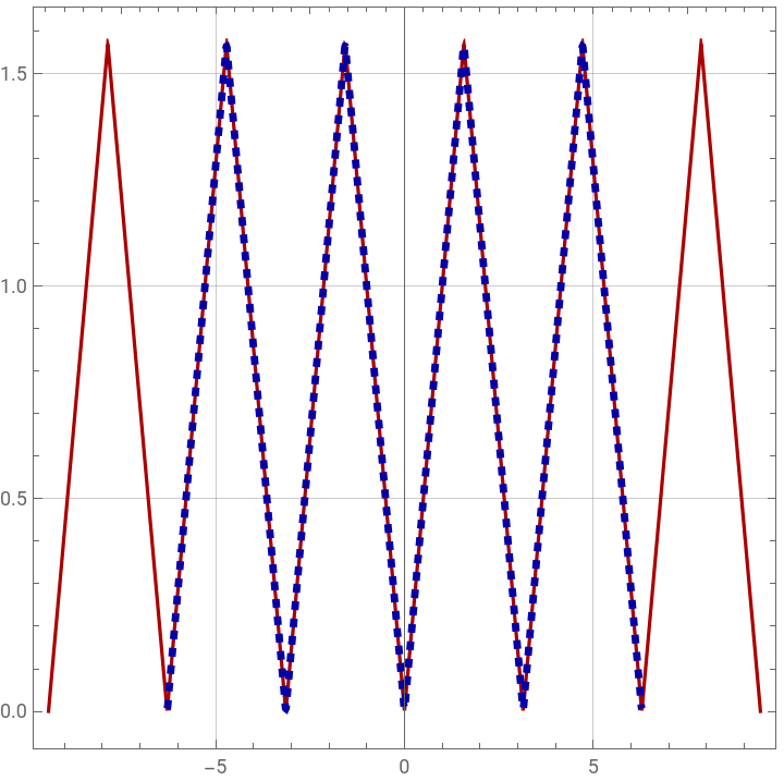
Superposing both plots: the function f(t) in red and its Fourier series approximation in dashed blue
In[]:=
Show[plt1,plt2,PlotRange{{-3Pi,3Pi},{0,Pi/2}}]
Out[]=
Using FourierSeries built-in command, we get the Fourier series approximation of f(t) (plotted in dashed green)
Superposing both plots: the function f(t) in red and its Fourier series approximation, obtained using FourierSeries, in dashed green