Estimating Planetary Perihelion Precession
Estimating Planetary Perihelion Precession

Making the simplified approximation that planets move in an isotropic central potential and applying conservation of angular momentum, the planetary equations of motion reduce to one-dimensional and become exactly soluble. In this simple picture, the rate of perihelion precession can be calculated to arbitrary precision. Applying methods introduced in[1], we obtain a "big equation" for the precession rate of an orbit's perihelion. Using data from[2] and the pseudopotential formulation of[3, 4], we determine values for all unknowns (see Details).
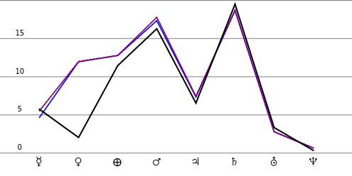
Substituting all determined coefficients for all planets into the big equation, we finally obtain precession predictions, which closely match those of[3, 4]. From the convergence graphs we see that, except with Mercury, a zero-order or first-order approximation is usually accurate enough. After calculating classical precession, it becomes possible to calculate the tiny additional anomalous precession by applying the same formulas on a gravitational central potential derived from general relativity[5].
Planet symbols: Mercury , Venus , Earth , Mars , Jupiter , Saturn , Uranus , Neptune .
☿
♀
♂
♃
♄
⛢
♆
Details
Details
As the computations in this Demonstration show, derivation of the big equation is relatively simple and fast when applied to a Hamiltonian of the form
H
ω
1
2
2
p
2
q
∞
∑
n=3
ϵ
n
n
q
where both and have the dimension of angular momentum. Per our ansatz for the phase space trajectory, the expansion parameter is then
2
p
2
q
α==
2
β
2H
ω
All gravitational pseudopotentials need to be transformed to the form of equation (1). The effective Hamiltonian for a particular planet can be expanded around a point according to
r
0
H
r
2
()
p
r
2m
r
0
∞
∑
n=2
n
v
n
r
0
Solar system data combined with the pseudopotential formulation[3, 4] uniquely determines the parameters and . As in[1], we then apply a canonical transformation
r
0
v
n
r⟶q=
r-
r
0
k
p
r
p
r
v
n
ϵ
n
n
k
v
n
ω
k=
-1/4
(2m)
v
2
ω=
2/m
v
2
to put the Hamiltonian (2) into the form of (1) by determining and as many as necessary. Notice that transformation (3) always forces to equal , as in equation (1) and the parameter table. We also transform the equilibrium radius by the canonical transformation
ω
ϵ
n
ϵ
2
1/2
ρ==
r
0
k
r
0
Finally, we estimate energy from data by using the observed perihelion and aphelion values to compute a variable for the span between the extrema where =0. Then the equation
α
r
p
r
a
δr=-
r
a
r
p
p
r
δr=k(q(α,ϕ=0)-q(α,ϕ=π))
can be solved numerically for . This completes specification of the data transformation theory, which determines all parameters in the table, thus determining the annual precession rate.
α
Comparing the calculation of Fitzpatrick to the calculation presented here, the most striking difference is the number and type of required variables. Fitzpatrick requires only the sets of mean radii and planetary masses. In our estimation, these quantities go eventually into the formulation of the pseudopotentials. But we also need angular momentum and energy , which help to determine just how the orbit will deform away from a circular shape.
L
α
Taking a look at the comparison graph, we see that the energy-independent part of our approximation
δθ=1-=1-=1-=1-
L
2
ρ
2
k
L
2
()
r
0
-1/2
(2m)
v
2
L
2
()
r
0
L
mω
2
()
r
0
does an acceptable job of matching the Fitzpatrick values, but the agreement is not exact for all planets. Mercury and Mars are noticeably different.
References
References
[3] R. Fitzpatrick, An Introduction to Celestial Mechanics, New York: Cambridge University Press, 2012.
[4] R. Fitzpatrick, "Perihelion Precession of the Planets," Newtonian Dynamics, 2011 (Sep 28, 2016). farside.ph.utexas.edu/teaching/336k/Newtonhtml/node115.html.
[5] A. Einstein, "Erklärung der Perihelionbewegung der Merkur aus der allgemeinen Relativitätstheorie." Sitzungsberichte der Königlich Preußischen Akademie der Wissenschaften, 1915 pp. 831–839. (Sep 27, 2016) einsteinpapers.press.princeton.edu/vol6-doc/261. English translation: einsteinpapers.press.princeton.edu/vol6-trans/128?ajax.
External Links
External Links
Permanent Citation
Permanent Citation
Brad Klee
"Estimating Planetary Perihelion Precession"
http://demonstrations.wolfram.com/EstimatingPlanetaryPerihelionPrecession/
Wolfram Demonstrations Project
Published: September 30, 2016