Numerical Inversion of Laplace Transforms
Authors: Housam Binous and Ahmed Bellagi
Numerical Inversion of Laplace Transforms
Authors: Housam Binous and Ahmed Bellagi
Authors: Housam Binous and Ahmed Bellagi
Acknowledgement :
Rice and Do, Applied Mathematics and Modeling for Chemical Engineers, Wiley, 1995.
Rice and Do, Applied Mathematics and Modeling for Chemical Engineers, Wiley, 1995.
The inversion of Laplace transforms is performed using two methods : (1) the Zakian method and (2) the Fourier series approximation . Results are in agreement with analytical solutions obtained using the built-in function of Mathematica : InverseLaplaceTransform . The Zakian method presents problems for transcendental functions . The Fourier series gives better results when dealing with oscillating functions .
The Fourier Series Approximation
In[]:=
Off[General::"spell1"]
Analytical Solution using the built-in function of Mathematica: InverseLaplaceTransform
In[]:=
F[s_]:=1/(s^2+1)
In[]:=
fexact[tt_]:=Evaluate[InverseLaplaceTransform[F[s],s,tt]]
In[]:=
fexact[t]
Out[]=
Sin[t]
In[]:=
plt1=Plot[fexact[t],{t,0,18},PlotStyleRGBColor[1,0,0],Frame->True,GridLines->Automatic,AspectRatio->1,FrameLabel->{Style["t",14],Style["f(t)",14]},ImageSize->350{1,1}]
Out[]=
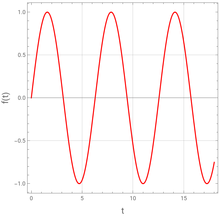
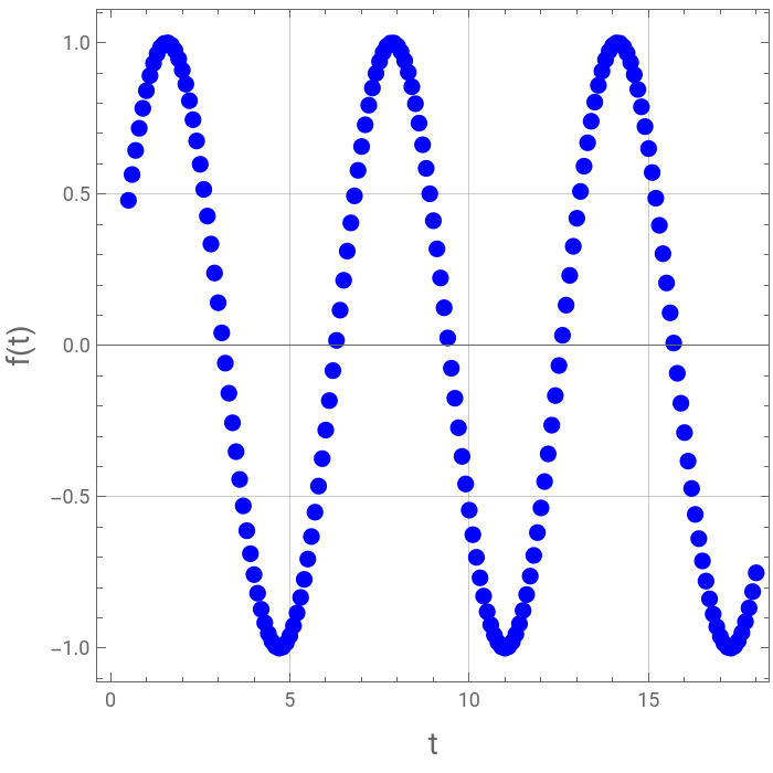
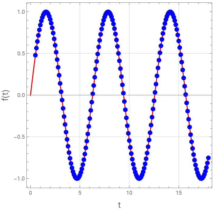
Numerical Solution using the Fourier Series Approximation gives the same result as the exact solution
In[]:=
t=Table[i,{i,0.5,18,2}]
Out[]=
{0.5,2.5,4.5,6.5,8.5,10.5,12.5,14.5,16.5}
In[]:=
fexact[t]//Chop
Out[]=
{0.479426,0.598472,-0.97753,0.21512,0.798487,-0.879696,-0.0663219,0.934895,-0.711785}
In[]:=
Er=10^-8;
In[]:=
σ0=0.001;
In[]:=
T=50;
In[]:=
σ=σ0-Log[Er]/(2T)
Out[]=
0.185207
In[]:=
finv=Exp[σt]/T12F[σ]+(Re[F[σ+kPiI/T]]Cos[kPit/T]-Im[F[σ+kPiI/T]]Sin[kPit/T])
2000
∑
k=1
Out[]=
{0.479426,0.598471,-0.977532,0.215118,0.798484,-0.8797,-0.0663283,0.934886,-0.711799}
In[]:=
TableForm[Transpose[{t,fexact[t],finv}]]//Chop
Out[]//TableForm=
0.5 | 0.479426 | 0.479426 |
2.5 | 0.598472 | 0.598471 |
4.5 | -0.97753 | -0.977532 |
6.5 | 0.21512 | 0.215118 |
8.5 | 0.798487 | 0.798484 |
10.5 | -0.879696 | -0.8797 |
12.5 | -0.0663219 | -0.0663283 |
14.5 | 0.934895 | 0.934886 |
16.5 | -0.711785 | -0.711799 |
In[]:=
t=Table[i,{i,0.5,18,0.1}];
In[]:=
finv=Exp[σt]/T12F[σ]+(Re[F[σ+kPiI/T]]Cos[kPit/T]-Im[F[σ+kPiI/T]]Sin[kPit/T]);
2000
∑
k=1
In[]:=
plt2=ListPlot[Transpose[{t,finv}],PlotStyle{PointSize[0.025],RGBColor[0,0,1]},Frame->True,GridLines->Automatic,AspectRatio->1,FrameLabel->{Style["t",14],Style["f(t)",14]},ImageSize->350{1,1}]
Out[]=
In[]:=
Show[plt1,plt2]
Out[]=
The Zakian Method
Analytical Solution using the built-in function of Mathematica: InverseLaplaceTransform
In[]:=
t=.;
In[]:=
F[s_]:=1/(s^2(s+1)^2)
In[]:=
fexact[tt_]:=Evaluate[InverseLaplaceTransform[F[s],s,tt]]
In[]:=
fexact[t]
Out[]=
-t
t
In[]:=
plt1=Plot[fexact[t],{t,0,10},PlotStyleRGBColor[1,0,0]]
Out[]=
Numerical Solution using the Zakian method gives the same result as the exact solution
In[]:=
α={1.28376767510^1+I1.666063445,1.22261320910^1+I5.012718792,1.0934303110^1+I8.40967312,8.77643472+I1.1921853910^1,5.22545336+I1.5729529010^1};
In[]:=
K={-3.6902082110^4+I1.9699042610^5,6.1277025210^4-I9.5408625510^4,-2.8916562910^4+I1.8169185310^4,4.6553611410^3-I1.90152864,-1.1874140110^2-I1.4130369110^2};