Wolfram Cloud Document

"Figure 0. The hero animation. A stylised spacecraft sits inside an Alcubierre bubble travelling at v = c. The cyan grid shows how the warp field lifts and bunches the local coordinate mesh; the translucent blue sphere is the bubble surface; the magenta ring at the equator is where the exotic matter (negative energy density) lives. Engine wake, starfield, and orbiting camera are just for atmosphere — the geometry, the grid, the ring and the spacecraft pose are computed from the analytic Alcubierre metric every frame. The full-size version of the same animation is in Section 5b below."

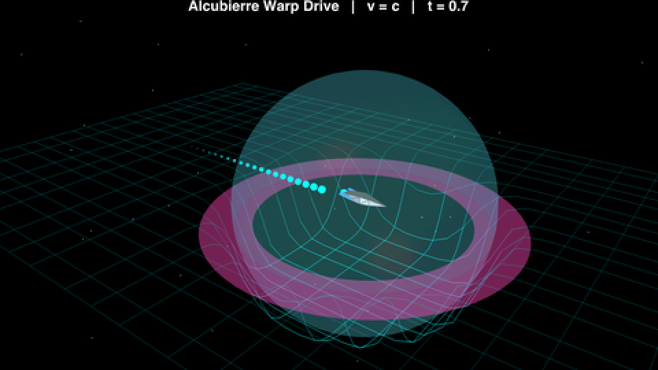
A symbolic-tensor playground for general-relativistic warp bubbles — from the Alcubierre metric to subluminal Bobrick–Martire shells, with native Einstein tensors, geodesics, and animated spacetime distortions. All analysed and compared by Claude.

Claude (Anthropic) with some guidance — github.com/mthiel74/WarpDrives

Abstract

Warp drives are the most science-fiction-sounding object in classical general relativity. In Alcubierre's 1994 construction, a spacecraft sits inside a flat "bubble" of spacetime that contracts the geometry in front of it and expands the geometry behind it. Locally the ship never moves faster than light — but the bubble itself can carry the ship across arbitrary coordinate distances in arbitrarily short coordinate times. The catch is the stress-energy: the metric requires a region of negative energy density in the bubble wall. This notebook ports the WarpDrives Python package into Wolfram Language packages and shows what symbolic-tensor machinery and DensityPlot / NDSolve buy you on this material: a working Einstein tensor in three lines, animated bubble fly-bys, geodesics that get swept up by the warp field, and side-by-side visualisations of the six metric families in the literature (Alcubierre 1994, Natário 2002, Van Den Broeck 1999, White toroidal, Bobrick–Martire 2021, Lentz 2021).

Status — hypothetical physics, not engineering. Every metric discussed below is a mathematical solution of Einstein's field equations in the reverse sense: one prescribes a desired geometry

μν

and reads off the stress-energy tensor

μν

/(8πG) that would be required to source it. No known substance produces the resulting

μν

. In particular, all superluminal warp metrics treated here (Alcubierre, Natário, Van Den Broeck, White, and the superluminal Lentz branch) violate the null energy condition (NEC), so they require exotic matter — regions of negative energy density as measured by some observer. Classical matter (dust, fluids, electromagnetic fields, scalar fields with canonical kinetic terms) cannot supply this; it is forbidden by every classical energy condition. Quantum field theory does permit small, transient negative energy densities (the Casimir effect, squeezed vacuum states), but the Ford–Roman quantum inequalities (1996) and Pfenning–Ford's bubble-specific bound (1997) show that the negative-energy budget for an Alcubierre bubble of macroscopic size scales catastrophically: a bubble of radius ~100m moving at

requires a wall thinner than the Planck length and a total negative mass-energy of order

grams — of order a billion times the baryonic mass of the observable universe (~

g), with the opposite sign. Even granting the matter, superluminal bubbles develop horizons (Finazzi, Liberati & Barceló 2009) that disconnect the ship from the front wall and exhibit semiclassical instabilities on timescales comparable to or shorter than the Planck time. The genuinely subluminal proposal in this notebook (Bobrick–Martire 2021) is the only one that can satisfy the weak and null energy conditions, but it still demands astrophysical energy densities; the Lentz 2021 hyper-fast soliton was originally advertised as positive-energy, but subsequent analyses suggest the construction still violates the classical energy conditions. Treat what follows as differential geometry of conceivable spacetimes, not a propulsion roadmap.

Getting started

Every figure and animation below is already rendered, so the post reads top-to-bottom in the browser — the animated GIFs embedded in each Output cell play directly in the Wolfram Community viewer. If you'd like to rerun or tweak any of them locally, the Input cell above each figure contains the exact call. Everything needed sits in a single self-contained package, WarpBubbleSim.wl (~37 KB, attached to this post). Drop it next to the notebook, evaluate the cell below once, and every public symbol used later (AlcubierreMetric, EinsteinTensor, CheckAllConditions, IntegrateGeodesic, …) becomes available:

SetDirectory[NotebookDirectory[]];Get["WarpBubbleSim.wl"];(*onefile(~37KB),66publicsymbols(64functions+EvalAt+NSamplesoptions)coveringshapefunctions,sixwarpmetrics,Christoffel/Riemann/Einsteintensors,ADMtools,energyconditions,geodesics,plottinghelpers.*)

Source repository (Wolfram + Python ports side by side): github.com/mthiel74/WarpDrives.

1. What is a warp drive?

In special relativity nothing locally outpaces light, and that sets a hard ceiling on travel times: at half the speed of light, the nearest star is still nine years away. General relativity is softer. Once spacetime can curve, the question "how fast did you travel?" splits into two questions — how fast did you move with respect to the local geometry (still bounded by c), and how fast did the geometry itself rearrange around you? Cosmology answers the second question routinely: distant galaxies recede from us superluminally because the universe is expanding, even though no individual galaxy moves faster than light through its own neighbourhood.

Miguel Alcubierre asked in 1994 whether the same trick can be played locally and on demand. The answer is yes: a sufficiently inventive metric can carry a flat-space "bubble" across the universe at any chosen

by contracting space in front of the bubble and expanding space behind it. The price tag, as we'll see in Section 9, is steep. But the geometry itself is surprisingly clean and admits a famously short closed form:

(dx-

)dt)

where

is the bubble's coordinate velocity,

its centre, with trajectory

(t)=

∫

(t')dt'

and

is the Euclidean distance from the bubble centre on the spatial slice

(x-

)

so a static observer at fixed

(x,y,z)

sees

shrink linearly to zero as the bubble flies past, then grow back. The shape function

)

is what gives the bubble a finite extent; mathematically it can be any smooth scalar with the asymptotic behaviour

f(0)=1,

lim

r∞

f(r)=0

Inside the bubble (

≤R

f≈1

) the line element collapses to

(dx-

dt)

, which is just Minkowski space written in coordinates that are boosted at velocity

— no curvature, no acceleration, the spacecraft sails along a straight worldline. Outside the bubble (

>>R

)

is essentially zero and the metric is again Minkowski. All the curvature and exotic-matter cost is concentrated in the wall region where

)

transitions from 1 to 0.

Alcubierre's original shape function is the Tanh sandwich

f(r)=

tanh(σ(r+R))-tanh(σ(r-R))

2tanh(σR)

with two free parameters:

sets the bubble radius,

controls the wall thickness (

σ∞

gives a hard step,

σ0

smears the wall over all of space). This is the canonical choice but other smooth profiles work too — a Gaussian, a compact-support polynomial, a smoothstep — each with a different trade-off between wall sharpness and energy density:

Plot{TanhShape[r,1,8],GaussianShape[r,1,0.4],CompactPolynomialShape[r,1,0.4],SmoothStepShape[r,1,0.3]},{r,0,2.5},



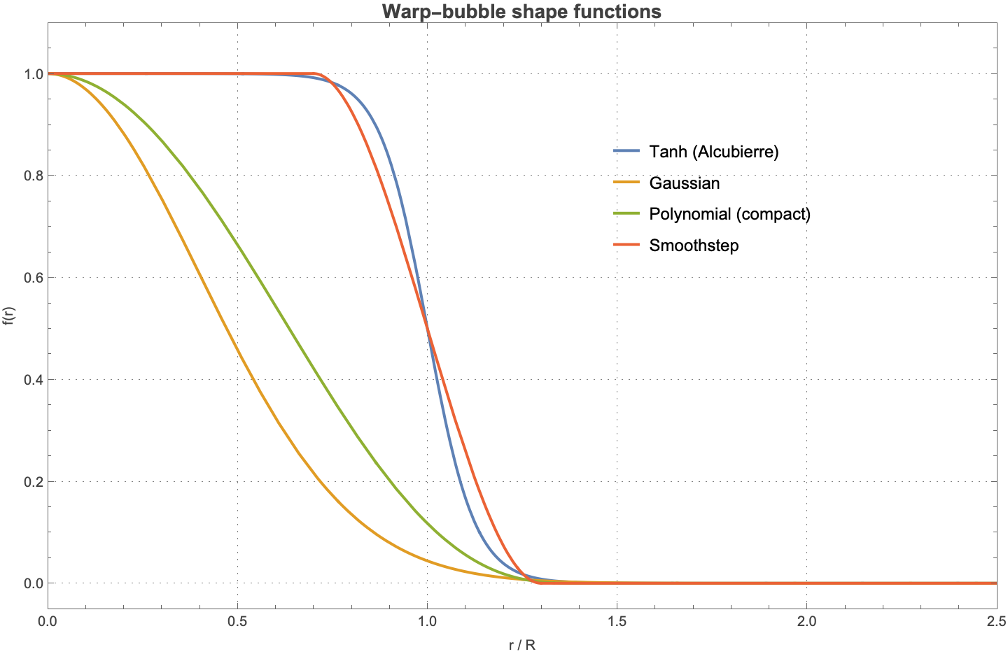
Four warp-bubble shape functions f(r) sharing the same boundary conditions f(0) = 1, f(∞) = 0. Tanh is the original Alcubierre profile; the others differ only in how sharply the wall falls off and whether the support is compact (CompactPolynomial, SmoothStep) or asymptotic (Tanh, Gaussian).

Each profile satisfies the same boundary conditions —

f(0)=1

f(∞)=0

— but they differ in how sharp the wall is and whether the support is compact. Sharper walls localise the exotic matter into a thinner shell at the cost of larger derivatives, which means more curvature, which means more energy. This is the first hint that the energy bill of a warp drive is essentially set by the geometry of the wall, not by the bubble's velocity.

2. The metric in ADM form

Every warp drive in the literature is most natural in the 3+1 ADM formulation. Foliate spacetime into spatial slices labelled by

; on each slice keep the spatial metric

; relate proper time on neighbouring slices by the lapse

; relate spatial coordinates between slices by the shift vector

. The line element splits into a temporal-distance piece and a spatial-displacement piece:

(

dt)(

dt)

Reading off matrix entries gives the standard 3+1 decomposition of the 4-metric:

with summation convention on the spatial indices

i,j∈{1,2,3}

and the spatial-metric raise/lower

. The inverse 4-metric has a similarly clean form:

-2

, which is exactly what ADMInverse[α, β, γ] in the package returns.

For Alcubierre's drive the ADM ingredients are spectacularly simple:

=(-

),0,0),α=1,

All the warp "weirdness" lives in that single

term — a unit-magnitude vector field along the direction of motion, modulated by the shape function so it switches on inside the bubble and off outside. In Wolfram, the helper AlcubierreMetric builds the full 4-metric symbolically:

g=AlcubierreMetric[{1,1,8},{t,x,y,z}];(*{v0,R,σ}*)MatrixForm@g

With

α=1

and

det(

)=1

the formula above gives

det(

μν

)=-1

everywhere, and Wolfram simplifies Det[g] back to that exact value:

Simplify@Det@AlcubierreMetric[{v,R,s},{t,x,y,z}](*->-1*)

3. Einstein tensor in three lines

This is where Wolfram earns its keep. In the Python port we built finite-difference Christoffel symbols, then finite-difference Riemann tensors, then finite-difference Ricci, all ~545 lines. In Wolfram the equivalent is a literal transliteration of the textbook formula because D differentiates symbolically. Recall the Christoffel symbols of the second kind:

αβ

μν



∂

βν

∂

αν

∂

αβ



In Wolfram this is one Table loop:

ChristoffelSymbols[g_,{t_,x_,y_,z_}]:=Module[{ginv=Inverse[g],dg=Table[D[g,c],{c,{t,x,y,z}}]},Table[(1/2)Sum[ginv[[m,n]](dg[[a,b,n]]+dg[[b,a,n]]-dg[[n,a,b]]),{n,4}],{m,4},{a,4},{b,4}]];

The Riemann tensor follows from the standard non-commutativity of covariant derivatives,

and Ricci is a single contraction, the Ricci scalar a second one:

Through the field equation

In Wolfram that's a one-liner. At a point on the bubble wall:

The same energy density rendered as a 3D surface brings out the wall structure. Figure 1 is a live Plot3D output cell, so in Mathematica or Wolfram Player you can click-and-drag to rotate the surface (the browser preview shows a default viewpoint).

4. Where space contracts, where space expands

So if you stand inside the bubble and look out the front porthole, distant galaxies appear to be rushing towards you; look out the back, they're racing away. The bubble itself "surfs" forward on its own private patch of contracting space. This is the qualitative picture you'll have heard described in popular accounts — and the picture above is its actual mathematical content.

5. The bubble in motion

5b. Putting a spacecraft inside the bubble

None of the geometry above changes if we put a "ship" inside the bubble — in Alcubierre's metric the interior is exactly flat Minkowski, so the spacecraft is in inertial free-fall and feels no acceleration even as the bubble accelerates across the galaxy. This makes for a striking visualisation, and because the package builds the metric symbolically we can render a fully self-consistent scene: the warp surface (a height field built from the shape function and the shift component), the translucent bubble, the magenta exotic-matter ring at the equator, the spacecraft mesh, an engine wake, and a star field. The camera orbits the bubble while travelling with it, so the spacecraft stays centred while the stars stream past:

The spacecraft itself is a small GraphicsComplex with 17 vertices and 30 triangular faces, plus two flat-quad nacelles drawn in glowing blue. The mesh is a literal port of the Python create_spacecraft() in generate_hero_animation.py:

The full mesh definition lives in build_hero_assets.wls, which also produces the GIF. Built into a 60-frame scene with an orbiting camera and a starfield, the result is the cover animation reproduced below at full size:

The 3D scene is striking but it makes the geometry hard to read. The complementary top-down view drops the height-field and lays everything flat: the energy density as the backdrop (red where exotic matter must live), the cyan grid still distorted by the shift field, and a triangular silhouette of the ship with two glowing nacelle dots. Annotations point at where space contracts and where it expands:

6. The grid being warped

7. Geodesics: getting swept up by a warp bubble

8. Six warp drives in one figure

The six metric families are mathematically distinct even though they share the same broad qualitative picture. In ADM form, each one differs only in the choice of lapse, shift, and spatial metric:

• Van Den Broeck keeps Alcubierre's shift but multiplies the spatial metric by a position-dependent conformal factor:

and pick the shell-region lapse, shift, and spatial-metric perturbations to satisfy the energy conditions. The key result is:

i.e. once the bubble is forced to move slower than light, ordinary positive-energy matter is enough to source it.

• Lentz uses a soliton ansatz with hyperbolic relations between lapse and shift, built from

and tied to an electromagnetic / plasma source via Einstein–Maxwell–plasma equations. Whether the original construction is genuinely positive-energy is debated in the literature.

9. Why this is hard: energy conditions

The classical energy conditions are coordinate-invariant statements about which kinds of stress-energy are "reasonable". Four of them are standard. The weak energy condition (WEC) says any timelike observer measures non-negative energy density,

The strong energy condition (SEC) controls the trace-reversed combination,

For ordinary matter — dust, photons, fluids, electromagnetic fields — all four are obviously satisfied. For an Alcubierre bubble at superluminal speed all four are violated, which is the rigorous statement of "requires exotic matter". The package ships sampling-based checkers for all four conditions; applied to a wall point of the v=c Alcubierre bubble (the option EvalAt substitutes coordinates after symbolic differentiation so the random observer sampler operates on a numerical metric):

Bobrick & Martire's 2021 paper showed something striking about this picture: drop the requirement of superluminal speed and the energy conditions can be respected. Subluminal positive-energy warp drives exist. They still cost an enormous amount of energy (orders of magnitude above any human energy budget), but the matter content is in principle sourceable by ordinary fields:

This is the clearest path forward in the literature: instead of trying to engineer exotic matter, find geometries which require none, even if the resulting drive is slower-than-light. None of this rescues warp drives from being hypothetical objects — even subluminal positive-energy constructions demand stress-energy distributions far outside any matter humans know how to assemble, and the energy budgets remain many orders of magnitude beyond global energy production. The value of writing the metrics down is not that they are buildable, but that they sharpen what general relativity does and does not forbid: causality and the field equations alone do not rule out faster-than-light effective travel; what rules it out, in practice, is the matter sector.

10. Implementation notes

11. What I take away

12. References

• M. Alcubierre (1994), "The warp drive: hyper-fast travel within general relativity", Class. Quantum Grav. 11, L73. doi:10.1088/0264-9381/11/5/001.
• J. Natário (2002), "Warp drive with zero expansion", Class. Quantum Grav. 19, 1157. arXiv:gr-qc/0110086.
• C. Van Den Broeck (1999), "A warp drive with more reasonable total energy requirements", Class. Quantum Grav. 16, 3973. arXiv:gr-qc/9905084.
• H. White (2011), "Warp Field Mechanics 101", presented at the 100 Year Starship Symposium (NASA Johnson Space Center technical report; non-peer-reviewed conference paper).
• A. Bobrick & G. Martire (2021), "Introducing Physical Warp Drives", Class. Quantum Grav. 38, 105009. arXiv:2102.06824.
• E. W. Lentz (2021), "Breaking the warp barrier: hyper-fast solitons in Einstein–Maxwell–plasma theory", Class. Quantum Grav. 38, 075015. arXiv:2006.07125.
• L. H. Ford & T. A. Roman (1996), "Quantum field theory constrains traversable wormhole geometries", Phys. Rev. D 53, 5496. arXiv:gr-qc/9510071.
• M. J. Pfenning & L. H. Ford (1997), "The unphysical nature of warp drive", Class. Quantum Grav. 14, 1743. arXiv:gr-qc/9702026.
• S. Finazzi, S. Liberati & C. Barceló (2009), "Semiclassical instability of dynamical warp drives", Phys. Rev. D 79, 124017. arXiv:0904.0141.
• Source code (Wolfram + Python ports): github.com/mthiel74/WarpDrives.

CITE THIS NOTEBOOK

Warp drives: symbolic tensor analysis of general-relativistic bubbles and energy conditions
by Marco Thiel
Wolfram Community, STAFF PICKS, April 27, 2026
https://community.wolfram.com/groups/-/m/t/3706027