Attributions
Attributions
Jacobian Conjecture, Eric W. Weisstein, July 20, 2026
This notebook downloaded from https://mathworld.wolfram.com/notebooks/Algebra/JacobianConjecture.nb.
For more information, see Eric's MathWorld entry https://mathworld.wolfram.com/JacobianConjecture.html.
©2026 Wolfram Research, Inc. except for portions noted otherwise
Counterexample Verification
Counterexample Verification
In[]:=
vars={x,y,z};f={z+(1+xy)(4+3xy),y+3xz+3x(4+3xy),2x-3y-z};jac=Outer[D,f,vars];pts=0,0,-,1,-,,-1,,;image[pt_List]:=Simplify[f/.Thread[varspt]];
3
(1+xy)
2
y
2
(1+xy)
2
y
2
x
3
x
1
4
3
2
13
2
3
2
13
2
images=image/@pts
Out[]=
-,0,0,-,0,0,-,0,0
1
4
1
4
1
4
In[]:=
Factor[Det[jac]]
Out[]=
-2
Visualization
Visualization
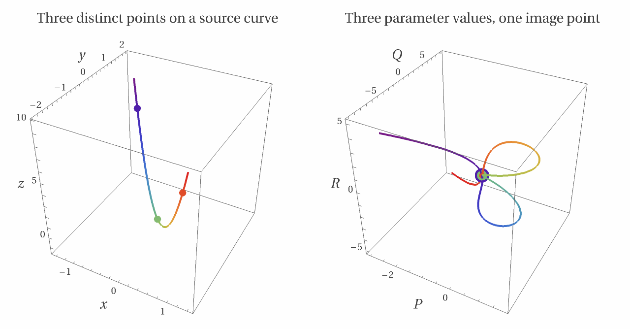
The full polynomial map sends three real dimensions to three real dimensions. This visualization follows a real curve through the three distinct source points and shows that its image passes through the same point at three parameter values.
In[]:=
sourceCurve[t_]:={t,-3t/2,(27t^2-1)/4};mappedCurve[t_]:=Factor[f/.Thread[vars->sourceCurve[t]]];collisionParameters={-1,0,1};sourcePoints=sourceCurve/@collisionParameters;mappedPoints=mappedCurve/@collisionParameters;collisionColors=ColorData["Rainbow"]/@Rescale[collisionParameters,{-1.15,1.15}];sourcePlot=Show[ParametricPlot3D[Evaluate[sourceCurve[t]],{t,-1.15,1.15},PlotStyle->Thick,ColorFunction->Function[{x0,y0,z0,t0},ColorData["Rainbow"][t0]],AxesLabel->(Style[#,Directive[14,Italic]]&/@{"x","y","z"}),PlotRange->All,PlotRangePadding->Scaled[0.12],BoxRatios->{1,1,1},SphericalRegion->True],Graphics3D[MapThread[{#1,PointSize[0.025],Point[#2]}&,{collisionColors,sourcePoints}]],PlotLabel->Style["Three distinct points on a source curve",14,FontFamily->"Times"],BaseStyle->FontFamily->"Times"];mappedPlot=Show[ParametricPlot3D[Evaluate[mappedCurve[t]],{t,-1.15,1.15},PlotStyle->Thick,ColorFunction->Function[{p0,q0,r0,t0},ColorData["Rainbow"][t0]],AxesLabel->(Style[#,Directive[Italic,14]]&/@{"P","Q","R"}),PlotRange->All,PlotRangePadding->Scaled[0.12],BoxRatios->{1,1,1},SphericalRegion->True],Graphics3D[MapThread[{#1,PointSize[#2],Point[First[mappedPoints]]}&,{collisionColors,{0.05,0.035,0.02}}]],PlotLabel->Style["Three parameter values, one image point",14,FontFamily->"Times"],BaseStyle->FontFamily->"Times"];Legended[GraphicsRow[{sourcePlot,mappedPlot}],Placed[SwatchLegend[collisionColors,Row[{Style["t",Italic]," ",#},BaseStyle->Directive[14,FontFamily->"Times"]]&/@collisionParameters,LegendLayout->"Row"],Bottom]]
Out[]=