ORIGINAL BOOK: Athanasios Paraskevopoulos (2023), Demystifying Epidemics: A Beginner’s Guide to Infectious Disease Modeling: Exploring Theories and Applications with Mathematica & R, Amazon. ISBN: 979-8868365027. https://a.co/d/9KXQkhu
I’m thrilled to announce the launch of my new book, “Demystifying Epidemics: A Beginner's Guide to Infectious Disease Modeling: Exploring Theories and Applications with Mathematica & R” Over the past 12 months, I’ve poured my passion for epidemiology into creating a comprehensive guide specifically tailored for undergraduate students.
This book is designed to be a comprehensive introduction to infectious disease epidemiology, demystifying complex concepts and terminologies right from the start. Starting with the foundational stones of infectious disease epidemiology, we embark on a journey into the realm of mathematical modeling. What sets this book apart is its unique dual focus on Mathematica and R, two powerful tools that bring their distinct strengths to the modeling process.
Whether you’re a beginner or have some experience in the field, this book progressively guides you through basic models to more intricate structures, providing a hands-on and practical approach to understanding and applying infectious disease modeling.
Mathematica and R enthusiasts will find tailored sections that leverage the strengths of each platform, making this book a valuable resource for anyone keen on exploring the intersection of epidemiology and data science.
I’m excited to share this educational journey with you! Grab your copy now and let’s unravel the mysteries of epidemics together!
Additionally, I’m actively seeking interest from public houses for this book. This is not a self-published endeavor; I envision it finding a home with a reputable publisher. Let’s make this collaboration a formal and impactful contribution to the field of infectious disease modeling
A data set on the prevalence of infection for an outbreak lasting 200 days in a population of 500 people is given, as shown in the table below .
In[]:=
Clear["Global`*"]
In[]:=
data={{10,19},{17,4},{24,5},{32,47},{36,38},{38,54},{41,84},{42,55},{47,116},{50,102},{52,126},{58,153},{59,164},{62,172},{63,177},{67,142},{68,158},{69,151},{75,155},{80,125},{81,116},{84,101},{87,106},{88,116},{94,85},{98,59},{102,67},{105,57},{114,59},{117,24},{118,39},{120,31},{128,36},{134,8},{140,7},{142,3},{147,20},{150,7},{155,2},{159,25},{163,2},{186,10},{191,17},{200,7}};dataTable=TableForm[data,TableHeadings->{None,{"Time","Number Infected"}}]
Out[]//TableForm=
Time | Number Infected |
10 | 19 |
17 | 4 |
24 | 5 |
32 | 47 |
36 | 38 |
38 | 54 |
41 | 84 |
42 | 55 |
47 | 116 |
50 | 102 |
52 | 126 |
58 | 153 |
59 | 164 |
62 | 172 |
63 | 177 |
67 | 142 |
68 | 158 |
69 | 151 |
75 | 155 |
80 | 125 |
81 | 116 |
84 | 101 |
87 | 106 |
88 | 116 |
94 | 85 |
98 | 59 |
102 | 67 |
105 | 57 |
114 | 59 |
117 | 24 |
118 | 39 |
120 | 31 |
128 | 36 |
134 | 8 |
140 | 7 |
142 | 3 |
147 | 20 |
150 | 7 |
155 | 2 |
159 | 25 |
163 | 2 |
186 | 10 |
191 | 17 |
200 | 7 |
In[]:=
pointsPlot=ListPlot[data,PlotStyle->PointSize[Medium],Frame->True,FrameLabel->{"Time (days)","Number Infected"},GridLines->Automatic,GridLinesStyle->LightGray,PlotRange->{{0,210},{-5,350}},BaseStyle->{FontSize->14},ImageSize->400]
Out[]=
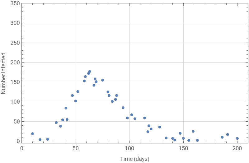
Plotting the dataset, this look like an epidemic curve for an outbreak starting with the introduction of one infected case . We have data points of the prevalence of infection spanning the entire duration of the epidemic (200 days), but not for every day . Define the simple SIR model and model input :
What are the best - fitting values for β and γ?
What are the best - fitting values for and ?
β
γ
Total size of population
n=500;
In[]:=
times=data[[All,1]]
Out[]=
{10,17,24,32,36,38,41,42,47,50,52,58,59,62,63,67,68,69,75,80,81,84,87,88,94,98,102,105,114,117,118,120,128,134,140,142,147,150,155,159,163,186,191,200}
Flu dataset
numberinfected=data[[All,2]]
Out[]=
{19,4,5,47,38,54,84,55,116,102,126,153,164,172,177,142,158,151,155,125,116,101,106,116,85,59,67,57,59,24,39,31,36,8,7,3,20,7,2,25,2,10,17,7}
In[]:=
ClearAll[β,γ]sireqns={s'[t]==-β*s[t]*i[t]/n,i'[t]==β*s[t]*i[t]/n-γ*i[t],r'[t]==γ*i[t]};initialConditions={s[0]==n,i[0]==1,r[0]==0};
In[]:=
sol=ParametricNDSolve[{sireqns,initialConditions},{s,i,r},{t,0,times},{β,γ}];
Extract the infected values from the solution
infectedValues=i/.sol;
In[]:=
objective[b_,g_]:=Norm[(infectedValues[b,g][times]-numberinfected)]^2bDom=Range[0,2,0.01];gDom=Range[0,1,0.01];res=Flatten[Table[{b,g,objective[b,g]},{b,bDom},{g,gDom}],1];Flatten[res[[PositionSmallest[res[[All,3]]]]]]//Most
Out[]=
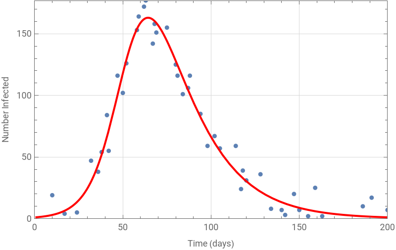
{0.16,0.05}
We can confirm visually that this parameter set produces a good model fit to the data, by overlaying the datapoints on a plot of the model output :
Set parameter values
{β,γ}={0.16,0.05};
Define the SIR model equations
sireqns={s'[t]==-β*s[t]*i[t]/n,i'[t]==β*s[t]*i[t]/n-γ*i[t],r'[t]==γ*i[t]};initialConditions={s[0]==n,i[0]==1,r[0]==0};
Solve the differential equations
sol=NDSolve[{sireqns,initialConditions},{s,i,r},{t,0,times}];
Extract the infected values from the solution
infectedValues=i/.sol[[1]];
Calculate the sum - of - squares (SSQ) value
ssq=Norm[infectedValues[Range[times]]-numberinfected]^2;

fitPlot=Plot[infectedValues[t],{t,1,200},PlotStyle->Red];Show[pointsPlot,fitPlot,PlotRange->All]
Out[]=
Based on our estimates parameter values, what would be the critical vaccination threshold required to prevent this epidemic, assuming an all - or - nothing vaccine with 75 % efficacy?
We can calculate the critical effective vaccination coverage as :
p
eff
1
R
0
1
β
γ
0.05
0.16
Since the all - or - nothing vaccine is only 75 % effective, we can calculate the critical vaccination threshold as :
p
c
p
eff
v
eff
0.69
0.75
only 8 % of the population are susceptible, 92 % of the population are vaccinated/immune
Plot the solutions
CITE THIS NOTEBOOK
CITE THIS NOTEBOOK
Demystifying Epidemics: A Beginner's Guide to Infectious Disease Modeling
by Athanasios Paraskevopoulos
Wolfram Community, STAFF PICKS, November 24, 2023
https://community.wolfram.com/groups/-/m/t/3070525
by Athanasios Paraskevopoulos
Wolfram Community, STAFF PICKS, November 24, 2023
https://community.wolfram.com/groups/-/m/t/3070525