In this project we have done benchmark computations for test 2D flow over cylinder in a flat channel in transient and steady cases. We have done a visual analysis for the solutions of Navier Stokes equations.
We have found that the benchmark computation for laminar flow are agreeable with the theoretical predictions.
We have found that the benchmark computation for laminar flow are agreeable with the theoretical predictions.
Navier-Stokes Equations
Navier-Stokes Equations
Navier-Stokes equations(N-S) are equations which can be uses to determine the velocity vector field that applies to a fluid,given some initial conditions. They arise from the application of Newton’s second law in combination with a fluid stress(due to a viscosity) and a pressure term. For almost, all real situations they result in a system of non linear partial differential equations; however with certain(such as 1-d motion) they can be modelled as linear differential equations. Usually however they remain non linear , which makes them difficult to solve , resulting in turbulence and unpredictability.
N-S equations are derived from:
N-S equations are derived from:
1
.Continuity equations
2
.Conservation of momentum:
dρ/dt+∇.(ρv)=0
ρ.Du/Dt=-∇p+∇.T+ρ.g
where gives the material derivative, ρ is the density, ∇. is the divergence, T is the stress tensor, g is acceleration due to gravity, and t is time.
The above equations together constitute the Navier-Stokes equations.
Due to complex nature of N-S equations, analytic solutions range from difficult to impossible, so the most common way to make use of them is through simulation and approximation. In the below sections we will examine the case of flow over cylinder for different test cases in steady and transient case.
D/Dt=∂/∂t+u.∇
The above equations together constitute the Navier-Stokes equations.
Due to complex nature of N-S equations, analytic solutions range from difficult to impossible, so the most common way to make use of them is through simulation and approximation. In the below sections we will examine the case of flow over cylinder for different test cases in steady and transient case.
Flow over cylinder
Flow over cylinder
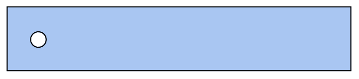
To visualise the flow , we first create a 2D case of cylinder in a flat channel as shown below.
In[]:=
H=.41;L=2.2;{x0,y0,r0}={1/5,1/5,1/20};Ω=RegionDifference[Rectangle[{0,0},{L,H}],Disk[{x0,y0},r0]];
We set up initial conditions for velocity and give the values for viscosity(ν) and initial input flow.
Here we have a time parameter in our input flow. It is necessary to determine the time dependence of drag and lift parameters for a half period of oscillation, as well as the pressure drop.
Here we have a time parameter in our input flow. It is necessary to determine the time dependence of drag and lift parameters for a half period of oscillation, as well as the pressure drop.
Initial conditions
In[]:=
K=400;Um=1.5;ν=10^-3;t0=.02;U0[y_,t_]:=4*Um*y/H*(1-y/H)*Sin[Pi*t/8]UX[0][x_,y_]:=0;VY[0][x_,y_]:=0;P0[0][x_,y_]:=0;
Create a Mesh
In[]:=
Show[BoundaryDiscretizeRegion[Ω],bmesh=HighlightMesh[BoundaryDiscretizeRegion[Ω,AccuracyGoal->5],{Style[1,Black],Style[2,None]}]]
Out[]=
Solving the Navier-Stokes equation
In[]:=
Do{UX[i],VY[i],P0[i]}=NDSolveValue·{{-μ,0},{0,-μ}}.u[x,y]+[x,y]+(u[x,y]-UX[i-1][x,y])t0+UX[i-1][x,y]*D[u[x,y],x]+VY[i-1][x,y]*D[u[x,y],y],·{{-μ,0},{0,-μ}}.v[x,y]+[x,y]+(v[x,y]-VY[i-1][x,y])t0+UX[i-1][x,y]*D[v[x,y],x]+VY[i-1][x,y]*D[v[x,y],y],[x,y]+[x,y]=={0,0,0}/.μν,{DirichletCondition[{u[x,y]U0[y,i*t0],v[x,y]0},x0.],DirichletCondition[{u[x,y]0.,v[x,y]0.},0≤x≤L&&y0||yH],DirichletCondition[{u[x,y]0,v[x,y]0},(x-x0)^2+(y-y0)^2r0^2],DirichletCondition[p[x,y]P0[i-1][x,y],xL]},{u,v,p},{x,y}∈Ω,Method{"FiniteElement","InterpolationOrder"{u->2,v2,p1},"MeshOptions"{"MaxCellMeasure"0.001}},{i,1,K};
∇
{x,y}
∇
{x,y}
(1,0)
p
∇
{x,y}
∇
{x,y}
(0,1)
p
(1,0)
u
(0,1)
v
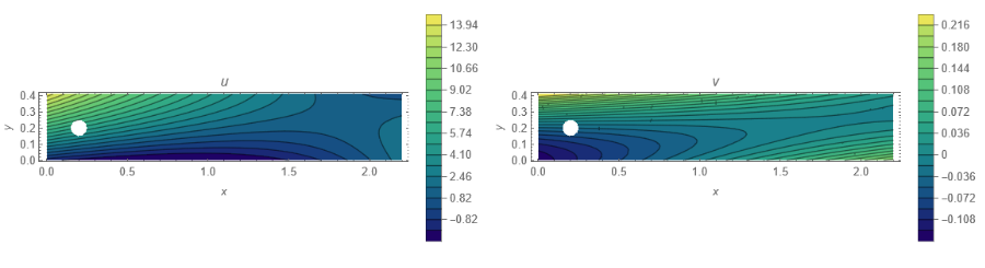
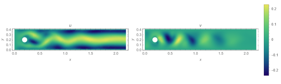
In the plots below we see the velocity profile shown below we see , the distribution near the surface of cylinder. There is no flow at the surface of cylinder known as stagnation points. We see a circulation trail behind the cylinder. We see a wake of vortices in this region.
This is due to negative pressure gradient. Further down the trail , the velocity just merges with the free stream velocity.
On the surface we have stagnation point. But there is a velocity profile as we go above in Y direction. This Phenomenon is known as Prandtl Boundary Layer.
These analysis were done for Reynold’s number in the range of 0 < Re < 100.
Contour Plots for U and V
In[]:=
Grid[{{ContourPlot[UX[K/2][x,y],{x,y}∈Ω,AspectRatioAutomatic,ColorFunction"BlueGreenYellow",FrameLabel{x,y},PlotLegendsAutomatic,Contours20,PlotPoints25,PlotLabelu,MaxRecursion2,PlotRangeAll,ImageSizeMedium],ContourPlot[VY[K/2][x,y],{x,y}∈Ω,AspectRatioAutomatic,ColorFunction"BlueGreenYellow",FrameLabel{x,y},PlotLegendsAutomatic,Contours20,PlotPoints25,PlotLabelv,MaxRecursion2,PlotRangeAll,ImageSizeMedium]}}]
Out[]=
Density Plots for U and V
In[]:=
Grid[{{DensityPlot[UX[K][x,y],{x,y}∈Ω,AspectRatioAutomatic,ColorFunction"BlueGreenYellow",FrameLabel{x,y},PlotPoints25,PlotLabelu,MaxRecursion2,PlotRangeAll,ImageSizeMedium],DensityPlot[VY[K][x,y],{x,y}∈Ω,AspectRatioAutomatic,ColorFunction"BlueGreenYellow",FrameLabel{x,y},PlotLegendsAutomatic,PlotPoints25,PlotLabelv,MaxRecursion2,PlotRangeAll,ImageSizeMedium]}}]//Quiet
Out[]=
Interpolation table for calculating pressure
In[]:=
dPl=Interpolation[Table[{i*t0,(P0[i][.15,.2]-P0[i][.25,.2])},{i,0,K,1}]];
Calculate the drag coefficient
In[]:=
cD=Table[t0*i,NIntegrate[-ν*-Sin[θ]Sin[θ][x0+rCos[θ],y0+rSin[θ]]+Cos[θ][x0+rCos[θ],y0+rSin[θ]]+Cos[θ]Sin[θ][x0+rCos[θ],y0+rSin[θ]]+Cos[θ][x0+rCos[θ],y0+rSin[θ]]*Sin[θ]-P0[i][x0+rCos[θ],y0+rSin[θ]]*Cos[θ]/.{rr0},{θ,0,2*Pi}],{i,1,K}];//Quiet
(0,1)
UX[i]
(1,0)
UX[i]
(0,1)
VY[i]
(1,0)
VY[i]
Evaluate the drag
In[]:=
drag[i_]:=drag[i]=θEvaluate-Cos[θ]P0[i]+,+-Sin[θ]-Sin[θ]Sin[θ]+,++Cos[θ]+,++Cos[θ]Sin[θ]+,++Cos[θ]+,+
1
5
Cos[θ]
20
1
5
Sin[θ]
20
1
1000
(0,1)
UX[i]
1
5
Cos[θ]
20
1
5
Sin[θ]
20
(1,0)
UX[i]
1
5
Cos[θ]
20
1
5
Sin[θ]
20
(0,1)
VY[i]
1
5
Cos[θ]
20
1
5
Sin[θ]
20
(1,0)
VY[i]
1
5
Cos[θ]
20
1
5
Sin[θ]
20
Plot the drag
In[]:=
Table[t0i->Plot[drag[i][θ],{θ,0,2Pi},FillingAxis],{i,1,K,10}]//TabView
Out[]=
0.02
0.22
0.42
0.62
0.82
1.02
1.22
1.42
1.62
1.82
2.02
2.22
2.42
2.62
2.82
3.02
3.22
3.42
3.62
3.82
4.02
4.22
4.42
4.62
4.82
5.02
5.22
5.42
5.62
5.82
6.02
6.22
6.42
6.62
6.82
7.02
7.22
7.42
7.62
7.82
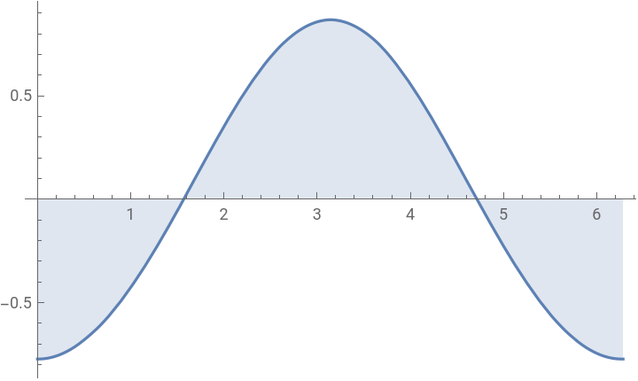
The Plot for the drag agrees with the theoretical prediction from Bernoulli’s theorem. We have used a numerical integration to solve for drag, method set to automatic.
Calculate the lift coefficient
In[]:=
cL=Table[t0*i,-NIntegrate[-ν*-Sin[θ]Sin[θ][x0+rCos[θ],y0+rSin[θ]]+Cos[θ][x0+rCos[θ],y0+rSin[θ]]+Cos[θ]Sin[θ][x0+rCos[θ],y0+rSin[θ]]+Cos[θ][x0+rCos[θ],y0+rSin[θ]]*Cos[θ]+P0[i][x0+rCos[θ],y0+rSin[θ]]*Sin[θ]/.{rr0},{θ,0,2*Pi}],{i,1,K}];//Quiet
(0,1)
UX[i]
(1,0)
UX[i]
(0,1)
VY[i]
(1,0)
VY[i]
Evaluate the Lift
In[]:=
lift[i_]:=lift[i]=θEvaluateSin[θ]P0[i]+,+-Cos[θ]-Sin[θ]Sin[θ]+,++Cos[θ]+,++Cos[θ]Sin[θ]+,++Cos[θ]+,+
1
5
Cos[θ]
20
1
5
Sin[θ]
20
1
1000
(0,1)
UX[i]
1
5
Cos[θ]
20
1
5
Sin[θ]
20
(1,0)
UX[i]
1
5
Cos[θ]
20
1
5
Sin[θ]
20
(0,1)
VY[i]
1
5
Cos[θ]
20
1
5
Sin[θ]
20
(1,0)
VY[i]
1
5
Cos[θ]
20
1
5
Sin[θ]
20
PLot Lift
In[]:=
ListPointPlot3D[Table[lift[i][θ],{i,1,K},{θ,0,2Pi,0.1}]]
Out[]=

The lift plot also agrees with the theoretical prediction. This gives us a check that FEM analysis can handle cases for even arbitrary shaped bodies.
Plot lift
Maximum and Minimum of Lift and Drag coefficient
Steady Flow case
Steady Flow case
Steady state just means that if the variables that define the behaviour of the system or the process are unchanging in time. For our case , this means the properties of fluid like temperature , pressure and velocity are unchanging with respect to time. This also means that the mass flow rate is constant in time. This means that there is no accumulation of mass in the system.
Setting up the Navier-Stokes equation
Here u represents fluid velocity in x direction and v represents fluid velocity in y direction.
Specify the PDE
What is a Dirichlet condition?
When imposed on a ordinary or partial differential equation ,it specifies the values that solution needs to take on the boundary. Here, we are doing just that, specifying velocity components at the ends to flat channel.
When imposed on a ordinary or partial differential equation ,it specifies the values that solution needs to take on the boundary. Here, we are doing just that, specifying velocity components at the ends to flat channel.
We set up the boundary conditions by setting up the inflow in x direction. On the upper and bottom part of the profile we specify no flow conditions. This is done by setting both u and v components zero in those regions. An outflow condition is on the right of the domain. Here the pressure is arbitrarily set to 0.
Specifying the Boundary conditions
As we know explicit closed forms(analytic solutions ) for N-S equations are rarely available. The finite element method(FEM) is a technique to solve PDE’s numerically.The advantages are it solves the PDE’s in any arbitrarily shaped region, it is also suited for large class of PDE’s.
To apply FEM we need:
To apply FEM we need:
1
.Discrete representation in the form of a mesh
2
.A partial differential equation
3
.Boundary conditions
In NDSolve , we can give the interpolation order, as the N-S equations are second order in u and v , first order in p , and set for increased accuracy.
The exact region need to be defined for NDSolve. NDSolve gives the numerical solution to the given differential equation.
The exact region need to be defined for NDSolve. NDSolve gives the numerical solution to the given differential equation.
Solve the equations with specifying the points , with increased accuracy and precision
We interpret the solution in the form of vector field, in the below contour plot , we see velocity distribution near the cylinder and far up stream. We see there is a change near the surface of cylinder ,the velocity near the upstream of cylinder is stopped , known as the stagnation point. Fluid elements passing above or below the cylinder increase the velocity, it turns out that the velocity is twice of the free stream velocity. Velocity along the surface of the cylinder is in tangential direction, i.e parallel to the direction of the flow.
We visualise the x velocity component profile near the cylinder and far field.
Contour Plot for velocity in X direction
We visualise the y velocity component profile near the cylinder and far field.
Contour Plot for velocity in Y direction
We see the pressure distribution near the cylinder and far field.
Contour Plot for Pressure
We see a vector field of velocity near the cylinder and the direction of flow.
Vector Plot for flow
We can calculate the lift and drag equations with
Setting up a function to calculate lift and drag around the cylinder
Integrate the force
Transient case
Transient case
Setting up the Navier stokes equation for transient case.
creating a ramp function for smooth inflow condition.
Setting up the boundary conditions
Setting up the initial conditions to 0
Time integrate the Navier stokes equation.
Find the maximum and minimum of x velocity range
For effective visualisation, extract the mesh from the solution
Extract mesh
Write a function to calculate vorticity
Load color data
Plot the contour plot for vorticity
Animate the contour plot
Conclusion
Conclusion
In this we have compared the different cases of flow over cylinder and calculated the several properties like lift , drag , vorticity.
We see that in employing Euler’s method for solving Hydrodynamics problem gives us results very close to the theoretical prediction for laminar flow model.
For future work we can look at turbulence modelling and consider approaches such as Large eddy simulations (LES) and compare it with techniques such as FVM.
Keywords
Keywords
◼
Fluid Dynamics
◼
Navier stokes equation
◼
FEM
◼
Turbulence
Acknowledgment
Acknowledgment
I’d like to thank my mentor Julián Laverde, for guiding my project, helping me review at every stage of the project and working with me on the project, motivating me on the project and also all the TA’s for helping me out in coding.
References
References