More than a year has elapsed since we released the multiway games blog. In such a short time, our exacting analysis could not diminish the general public’s love for puzzles and games, but neither have we been able to solve every last game or maze problem on the face of the earth. Another item for our analysis happened to be found in New York City, Fosun Plaza, Saturday, July 15, 2023. The Museum of Mathematics provided a few life-size mazes for their annual maths festival, including one with color-cycling rules that even managed to stump this humble author. Later in the evening, with computer tools from the games blog and air-conditioning from the hotel, the solution was found quickly and easily. In this sequel, we are concerned not just with one particular maze solution, but more generally, with what our tools can tell us about spaces of similar multi-state mazes. How difficult, comparatively, is this one example chosen by MoMath for public consumption? Are there any other interesting examples we should know about?
A Red, White and Blue multi-state maze
A Red, White and Blue multi-state maze
In the picture above, what have these patriotic youngsters gotten themselves into? The maze is a set of grid locations surrounded by colored edges. The rule for traversing the maze is that the explorer must sequentially step over a red edge, a white edge, a blue edge, and then continue cycling through red, white, and blue until the goal is reached after about twenty steps. Although the maze interior has sixteen locations, we shall see that only twelve are necessary for the shortest path solution. The maze itself can be drawn by reading edges and colors off the image above:
Out[]=
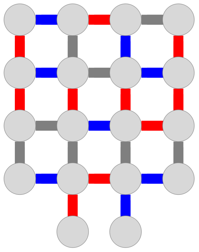
Starting at the entrance to the lower left, the first three steps are forced:
Out[]=

At the fourth step, it is possible to go either north or east. Neither of these choices is immediately a dead end because both have a white (or gray) edge which could be used for a next step. In fact, the state space is small enough to fully enumerate via breadth-first search (using NestWhileGraph):
Out[]=
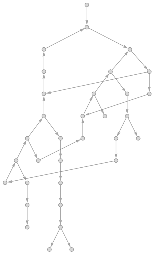
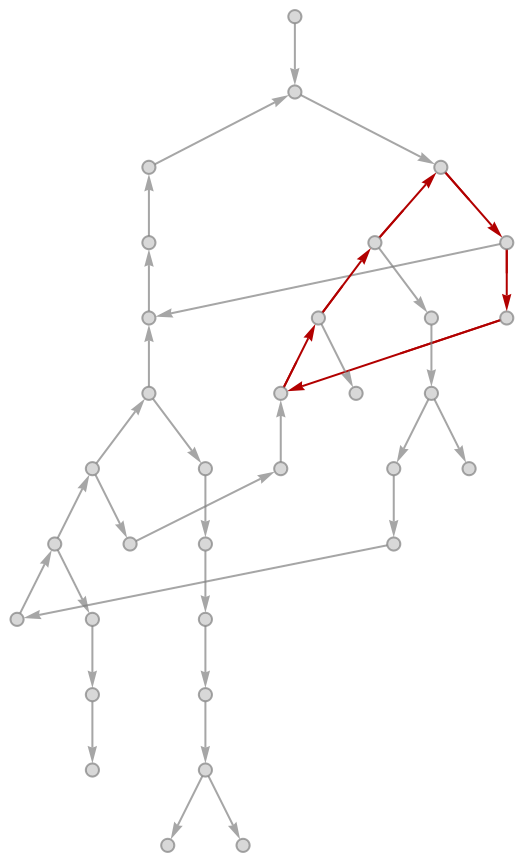
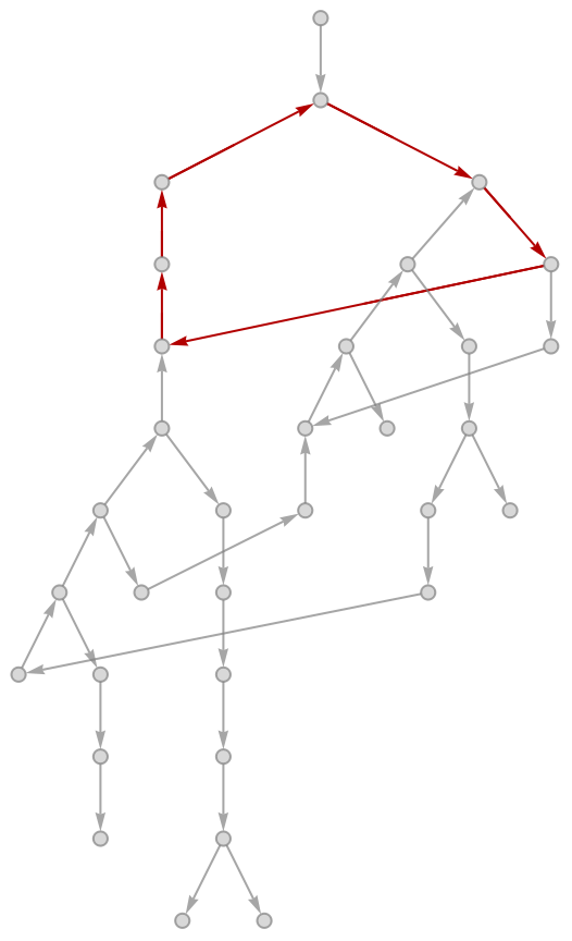
A maze’s resistance to being solved is partially a function of how many distinct loops it can throw its explorers into. Here we find four distinct alternatives, two of which branch immediately from the fourth step into the maze:
Out[]=
,
,
,
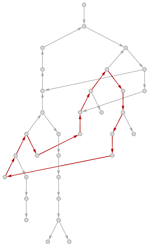
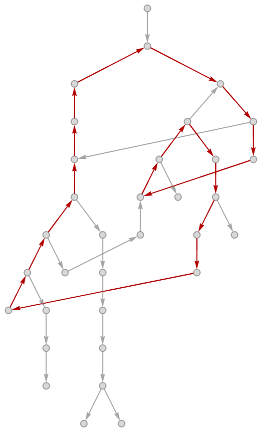
Is this maze even solve-able? Indeed it is, and we can find a unique shortest path from start to finish which requires only twenty-two steps in total:
solutions=FindPath[solutionsGraph,{5,2,Red},{5,3,Red},Infinity,All];
In[]:=
Length/@solutions
Out[]=
{22}
The solution can be plotted as:
Out[]=
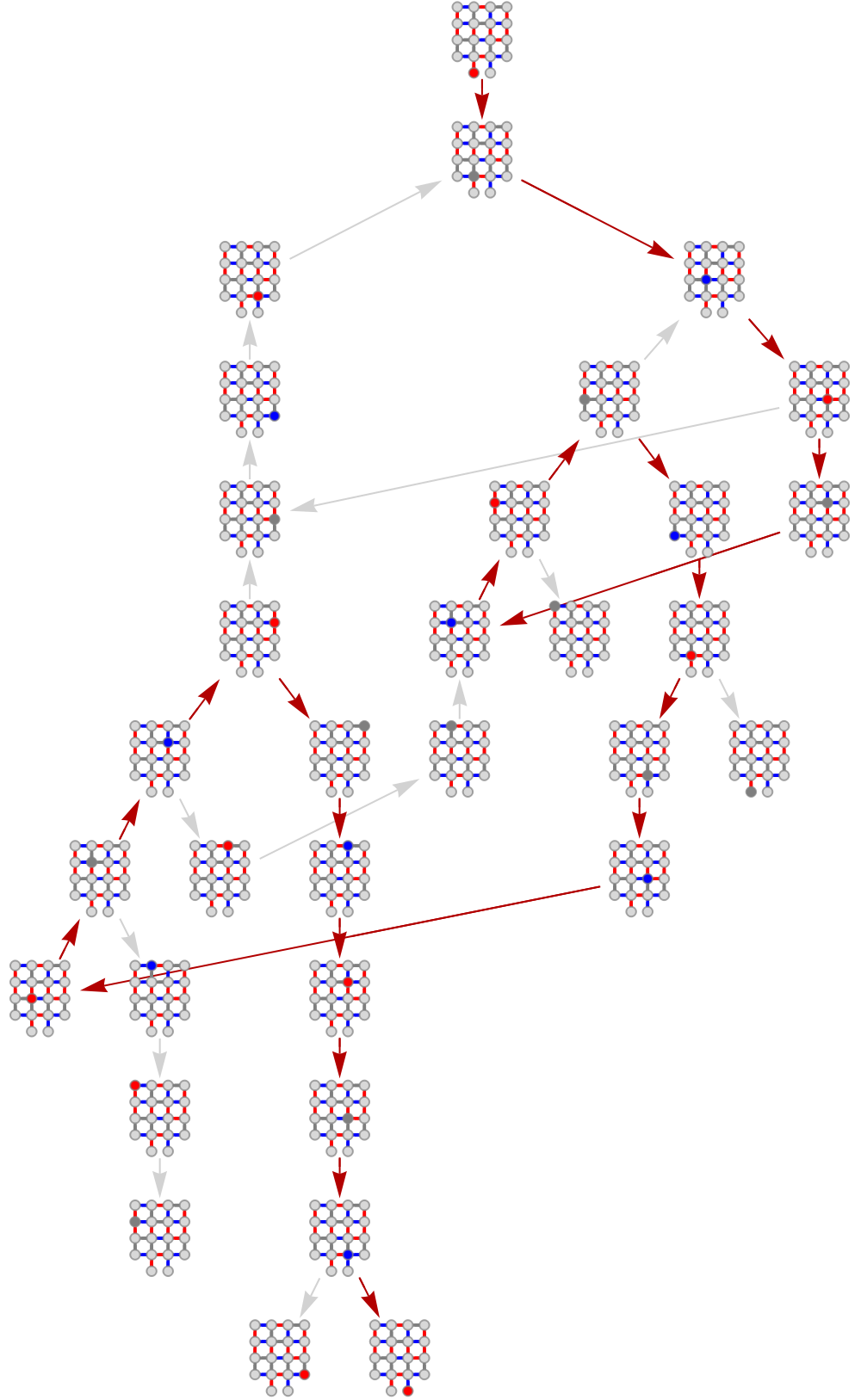
Once the solution is known, we can immediately notice that it doesn’t visit every grid location. Projecting out the state color, we find the following solution map in Cartesian space:
Out[]=
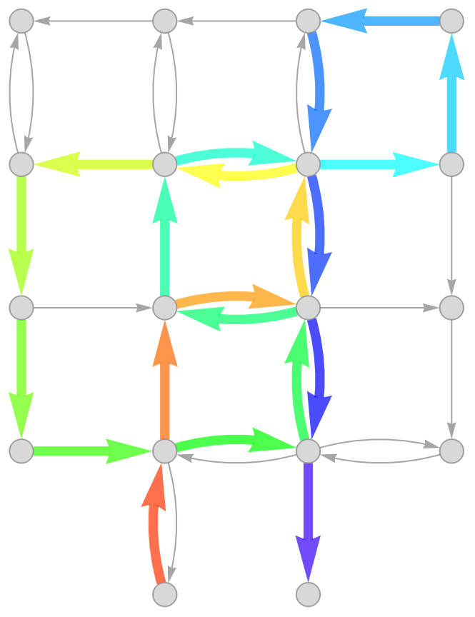
After eliminating four extraneous vertices, the number of loops in the state transition graph reduces from four to only one:
Out[]=
→
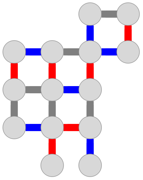

But the story of a maze’s difficulty is not told entirely by the count of loops. If dead ends are more difficult to notice, as they are before pruning extra sites, then it should be easier for maze explorers to unknowingly take a wrong turn. To make things more quantitative, let’s assume our explorer can remember all previous states, and refuses to visit any particular state twice. In practice, this restriction can be imposed by calling to MultiwayDeletionsGraph. The assumption of a self-avoiding walk effectively cuts apart loops in the game graph, leaving us with nice directed acyclic graphs:
The simplified graph on the right is obviously much easier to solve. There are only two dead ends, and each of these extraneous branches ends immediately after one erroneous step. In a more extensive search and analysis, we can’t examine each graph by eye. Instead, we can at least use DirectedAcyclicEvaluate to automate branch length counting as follows:
Comprehensive searching
Comprehensive searching
The 4×4 grid graph has 24 interior edges, thus allows a space of 282,429,536,481 three-colored multi-state mazes. Even if we restrict to have equal numbers of red, green, and blue edges, the total number of mazes still reaches the billions: 9,465,511,770. A 3×3 grid graph has only 12 interior edges, and if these are split evenly between red, green, and blue, then the total set of candidates has only 34,650 elements to test, not too many. Codes for the mazes can be calculated as follows:
For example, a randomly selected game graph is seen here:
Using colored Cartesian coordinates to indicate individual states, the corresponding state transition graph can be drawn as:
The total number of cyclic candidates is only 2088, small enough to compute and store state transition diagrams. Doing so, we can also gather codes into symmetry classes, which reduces the number of candidates by another factor of 24:
The number 24 comes from 8 symmetries of the square times 3 cyclic permutations of the colors red, blue, and green. In one case 48 codes are gathered together, possibly because the cyclic subgraph of the s.t.g. is relatively small and collides between otherwise unrelated mazes. We can take a characteristic element from each set and re-group these by cycle count:
Two of the 2-cycle candidates are very similar in terms of structure:
Again we can tree-ify the s.t.g. using MultiwayDeletionsGraph:
The astute reader will quickly realize the vertex-deletion trick from earlier also applies here, after which the state transition graphs simplify to isomorphism:
Here is the other s.t.g. with two distinct cycles:
The structure is similar here, again with two six-cycles and a few hanging branches. When it’s not entirely easy to see where to start and where to end, we can simply tree-ify from all valid starting points:
Finally, let’s automate analysis over the remaining set of 1-cycle candidates. Here we’ve added an extra depth variable, which should indicate roughly how much of the maze is actually necessary to obtain a solution:
Plotting solution graphs for the first few promising mazes, we notice many are not good because they end up with similar solutions on parallel branches:
We can filter these out and plot again:
Random Sampling
Random Sampling
In the previous section we gained some intuition how to filter mazes, and can now apply this intuition when random sampling from the set of more than 9 billion balanced 4x4 maze graphs. A random game can be obtained as follows:
The corresponding state transition graph is acyclic:
An acyclic s.t.g. is fairly typical, and we can test to see cyclic graphs show up with roughly 1 in 10 odds:
Aiming for about 10,000 cyclic candidates, we can start with a gross sample size of 100,000 codes, and start filtering the results from there:
As before, we can group these by cycle count:
First let’s check the outlier at 12 cycles. None of it’s unique solutions are significant in terms of length:
After this non-result we checked four cycles and three cycles, filtering mainly for tree depth. Details are omitted here, but one obvious outlier in the three-cycle set with code 50,355,573,788 had an s.t.g. of unusually large depth. It can be drawn out as:
Projecting the winning solution into Cartesian space and hue-coloring to give a sense of time, we can finally see that the unique solution visits all 16 interior vertices:
The real advantage of our newly discovered maze is that it has a long solution path at 30 steps, and there are no obvious simplifications to reduce apparent difficulty. If you want to try it out for yourself, just ignore the solution above and start on green here:
Limits and fixed points (briefly)
Limits and fixed points (briefly)
In the preceding analysis, we have assumed special memory powers for our maze explorers, powers which can’t be reliably guaranteed in a real world experiment. An essentially opposite assumption is that explorers will retain no past recollection and choose randomly at every juncture. Tree-ification of the s.t.g cannot be done simply by self-avoiding walk. Consequently the explorer can get stuck infinitely looping in one cycle subgraph. But with random choosing and at least a few dead ends / exits in the maze, infinitely long walks should ultimately have zero probability.
Let’s start with a toy example, just to see what happens. Here is a phase-locked maze, which is exceptionally easy to analyze:
By phase-locked, we mean that one state transition diagram can be drawn in Cartesian space with a chosen phase coloring consistent with potentially-infinite cycling:
After ten steps, the pattern to the s.t.g. starts to become apparent:
The color of the first output depends on the color of the input, and output colors cycle through red, green, blue as the explorer continues to cycle. After every three steps, the s.t.g. has an another output of the same color. The inherent symmetry allows us to write down an easy equation to solve:
This equation basically says that there is a value summing over all outputs of the same color, and if the sum is normalized so that the first output has value one, then the final sum will be 8/7. Indeed, this solution can also be tested numerically to hundreds of digits of precision:
There is yet another way to find the connection to one-sevenths, which is to write down continuity equations from the maze and extract the so-called “payoff matrix” directly:
This matrix is very similar to what we would find for the game of rock-paper-scissors, because each row has a low, middle, and high value, and the rows themselves are related by cyclic permutation. The particular matrix elements in r.p.s. are more obviously fair:
For a slight diversion into almost-normal game theory, let’s introduce adversarial players who each choose a strategy in the form of a normalized vector with three positive components. The game is played by taking the “sandwich product” of the payoff matrix between the two strategy vectors. A number is then obtained, which determines the winner of the game. The fairness of a win-condition depends a lot on statistics associated to the payoff matrix. For example, here are histograms of the possible outcome values for our cycle maze and rock-paper-scissors when choosing random strategies bilaterally:
Rock paper scissors looks obviously fair with regard to reflection symmetry around zero. To make a game based on the cycle maze fair, the distribution of outcome values would need to be integrated to find a midpoint. The mutually opposed win condition could then be given as greater or less than the determined midpoint.
Returning to the main narrative, our typical mazes have one preferred input and one preferred output, so we are really only concerned with one matrix element. Again, this matrix element will tell us the probability of solving the maze when making only random choices at each branch point. For a brute force calculation of such a number, we can simply tree-ify the s.t.g to increasing depth:
Subjecting this sequence of graphs to DirectedAcyclicEvaluate, we can obtain a sequence of rational approximants for the maze’s random fairness:
As the loops are explored more thoroughly, a limit is traversed toward a fixed point where the number in question reaches a maximum value 1/168 ~ 0.005952... This answer can be computed analytically, again by solving a system of continuity equations:
What’s really happening with the solution is that every edge gets a weight, and then the output node takes its final weight from the immediate preceding edge. We can do similar for the MoMath maze, and obtain a random fairness value of 1/90:
This again indicates what we could have guessed by intuition, that the MoMath maze is slightly easier to solve than the other one we found by targeted searching.
Conclusion
Conclusion
We’ve shown how the tools from the WFR can be useful not only for solving pre-existing mazes, but also for searching maze spaces to find particularly challenging examples. Considering the state transition graph as a generic directed graph, possibly with cycles, we’ve also taken a step forward into the next necessary round of development. For a certain class of vertex functions, it is possible (even for a digraph with cycles) to obtain a payoff matrix which can also act effectively like a transfer matrix between input and output values. In the future it will be possible to have a function such as “DigraphEvaluate” (don’t worry, the name probably will not stick) which solves systems of equations to obtain vertex and edge weights. Before this can be done, more research needs to be done into which vertex functions are fully reversible and lead to uniquely determined systems of equations.
Acknowledgements
Acknowledgements
Ed Pegg originally informed me of multi-state mazes through his webpage here. We don’t presently know for sure, but the life-size, multi-state maze at MoMath was probably designed by Andrea Gilbert of clickmazes.com.
CITE THIS NOTEBOOK
CITE THIS NOTEBOOK
Maze solving at NYC Math Festival
by Brad Klee
Wolfram Community, STAFF PICKS, July 26, 2023
https://community.wolfram.com/groups/-/m/t/2977383
by Brad Klee
Wolfram Community, STAFF PICKS, July 26, 2023
https://community.wolfram.com/groups/-/m/t/2977383