Wolfram Cloud Document

CITE THIS NOTEBOOK: Simulating media's effects on inflation in a simple economy by Wolfram Emerging Leaders Program. Wolfram Community JAN 27 2023.

The Wolfram Emerging Leaders Program is a 4-month long, project-based program designed for gifted high school students to take a deep dive into a topic of their choice. Students work remotely in small groups to take their project from ideation to completion, with the guidance of Wolfram experts. Wolfram Emerging Leaders Program participants are selected from the Wolfram High School Summer Camp, which is open to talented, STEM-oriented students age 17 and under. This essay was written by:

◼

Matt Sprintson

◼

Karan Chakravarthy

◼

Stella Maymin

Abstract: This project explores the trading behavior of a simple market with both explicit and implicit inflation. In both cases, both cost-pull and demand-push inflation are at play, but in one case, sellers are naturally responding to changes in cost and demand, and in the other, sellers are pushed towards the market equilibrium through a "media" warning them about impending inflation.

Introduction

Imagine yourself as a child looking to earn a quick buck. Of course, with your plethora of business acumen, you analyze the market and decide that setting up a lemonade stand would be the most profitable endeavor. So, as a businessperson would do, you begin to pitch your idea to a group of investors. Then, when your parents eventually give in, you go to the store and buy the requisite ingredients.

Now, it’s been a few weeks, and your stand has made a good amount of money. You’re using $2 to purchase the ingredients and sell each glass for $4. After a while, you realize that people want to buy lemonade even after you’ve run out of ingredients. Rallying around your insatiable cupidity, you increase your prices and production. Then, after a few weeks, the cost of your inputs increases as well, forcing you to adjust your prices.

These processes, which economists dub cost-push and demand-pull inflation, will occur naturally as the money supply rises. As a business owner, you do not realize that people willing to buy your lemonade for more than $4 is not due to an increase in demand but only a decrease in the value of money.*

But imagine that, in an alternate universe, you watch the news with your father. The anchor is discussing “inflation,” which makes you excited — doesn’t everyone love balloons? But your father is less enthusiastic. He says that 10% inflation means you need to raise prices by 10% since the dollar is only worth 90% of what it was. So, you immediately raise your prices.

Inflation has had the same effect, but explicit inflation has occurred much faster than implicit inflation. In our project, we simulated the same market and found a similar result. When the value of money decrease, rational sellers naturally increase prices, though when media tells sellers about price increases, they adjust quicker and end up with higher prices.

*For our purposes, we assume that this lemonade stand is only open for a short period of time. i.e, we assume that all these actions happen in the short run, as most economists agree that money is not neutral in the short run. We do this because of the theory of monetary neutrality in the long run. That is, money can not change real variables like supply as input costs and output costs increase at the same rate. In our model, we act in the short run, as inflation impacts the supply of each seller.

Functions and how they Function

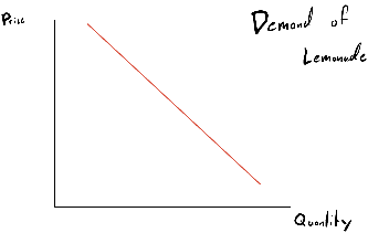
Demand

We began with the economic principles: a simple demand curve.

In[]:=

demandMax=150;demand[price_,sellerInventory_,buyerMoney_]:=Module[{demandRaw, tempDemand,itemsEnquered},demandRaw=Floor[demandMax-price];itemsEnquered = Floor[buyerMoney/price];If[demandRaw>sellerInventory,tempDemand = sellerInventory;,tempDemand = demandRaw;];If[tempDemand > itemsEnquered,Floor[buyerMoney/price],tempDemand]];

Then, Murphy's law applied, and we needed to make our code much more complicated. A simple demand structure with Quantity Demanded set as (150 - price) does not account for the amount of supply that the seller has. In other words, if a customer walked up to my lemonade stand and said, "I want to buy 75 lemonades!", I would reply with, "I only have 60." They would get Null lemonades, I would get Null money, and then no one would be happy. Instead, our function first creates a "demandRaw" and then compares it to the seller inventory. Then, we create a "itemsEnquered," which is just a silly way of saying "How much can I afford to buy?" At this point, we are able to compare the two: demandRaw and itemsEnquered. First, if we want to buy more than the seller has, we buy the entire stock. Subsequently, if we want to buy more than we can afford, we buy all that we can afford.

After that complicated process, the demand function leaves us with the amount of lemonade that the buyer is able and willing to buy (which is the literal definition of "demand").

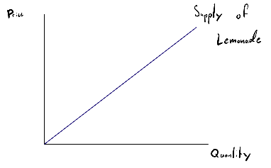
Supply

The supply function calculates how much of a product a seller will produce based on the current price. This function directly emulates a simple supply curve. The "costPerItem" refers to the price needed for a seller to create an item. This process is much less complicated than demand because the sellers will update their stock at the beginning of each round or time step.

In[]:=

supply[price_]:=(price)costPerItem = 50;

Associations

We used associations to represent the state associated with all of our buyers and sellers: state is an association of buyers and sellers.

Buyers are associated with two quantities:

◼

“items” - how much lemonade they have purchased

◼

“income” - how much money they have

Sellers are associated with ten different quantities:

◼

"key" - a variable that allows us to sort each seller based on price while not losing the original placement of the seller.

◼

“items” - how many items they have to sell

◼

“price” - the price at which they are selling a product

◼

“revenue” - the amount of money they have made before costs.

◼

“DSH” - the Demand-Supply heuristic which is the difference between the total number of items a buyer would buy and the number of items a seller is selling.

◼

“TotalCost” - the DSH times the price, or the implicit cost of under or overselling

◼

“profit” - the profit the seller makes in one cycle

◼

“prevPrice” - the previous price of the seller to help us decrease or increase the price with a reference point

◼

“prevProfit” - the previous profit of the seller to see if the change in price resulted in profit or loss

◼

"ldProfit" - the previous, previous profit of the seller to help in case the sellers are stuck between two prices.

In[]:=

Changing our Prices

The ChangePrice functions are used to determine the new price at which a seller will sell their product. We created multiple ChangePrice functions to represent different algorithms a seller might use to determine the price that might maximize their profit. Consequently, the ChangePrice functions take different inputs but all output a single new price. For our project, we used the ChangePrice3 function.

The ChangePrice1 function modifies the price solely based on the Demand-Supply Heuristic. Hypothetically, this would be the most efficient method to determine if a seller is above or below the market equilibrium. We decided not to use this model, as sellers are unlikely to know the aggregate demand of an economy.

Unlike ChangePrice1, the ChangePrice2 function also takes the one previous DSH as an additional input. If the DSH reaches a maximum or minimum, the previous 2 DSHs will likely be equal, in which case the price is not changed. Otherwise, the price changes similarly to ChangePrice1. Again, we decided to forgo this method as a seller is unlikely to know the exact equilibrium in an economy.

The ChangePrice3 function is the final model. ChangePrice3 compares the previous price and profit to the current price and profit. With this information, the function is able to alter the price accordingly. If the seller raised the price and their profits increased, then it would continue to increase the price, etc. In order to prevent the seller from simply changing between two unprofitable states, if the seller had the same previous price and new price, the method would compare the difference between the previous profits and the new profits and change accordingly.

In[]:=

ChangePrice1[oldPrice_, dsh_]:=Module[{newPrice,tempPrice},newPrice=If[Equal[dsh,0],oldPrice,If[dsh>0,oldPrice+1,oldPrice-1]];newPrice]

In[]:=

ChangePrice2[oldPrice_, dsh_,oldDSH_]:=Module[{newPrice,tempPrice},newPrice=If[Equal[dsh,0]||Equal[dsh,oldDSH],oldPrice,If[dsh>0,oldPrice+1,oldPrice-1]];newPrice]

In[]:=

ChangePrice3[oldPrice_, oldProfit_,currentPrice_,currentProfit_,items_,ldProfit_]:=Module[{newPrice},newPrice=If[oldProfit>=currentProfit,If[oldPrice>currentPrice,newPrice=currentPrice+4,newPrice=currentPrice-4],If[oldPrice>currentPrice,newPrice=currentPrice-4,newPrice=currentPrice+4]];If[newPrice == oldPrice,If[ldProfit >= currentProfit, newPrice = newPrice +4,newPrice = newPrice - 4]];If[currentProfit < 0 & items ==0, newPrice = newPrice +6];If[newPrice<=0, newPrice+7, newPrice, Print["UH OH!"]]]

The following method is only for examples within this computational essay.

We decided to increase the amount prices are changing to 4. For logic' sake, when a lemonade stand owner wants to increase their prices, they wouldn't likely increase their prices by $0.1 each time. For practicality's sake, it saves us computation time and we can watch the numbers increase faster.

Creating a simple market

The interact function is the most fundamental function in our program. This function allows buyers to purchase products from the sellers and represents one round of a buying-selling cycle. As mentioned previously, we used associations to represent the buyers and sellers. The interact function takes in the initial state in the form of an association and, after running, returns a new association with updated values of the buyers and sellers.

The interact function below is not used in our final code, but gives us a sense of how the internal mechanisms function before we add inflation.

Because we wanted to change the inputs in the association for each seller individually, we mapped through all the sellers in the association. The names of our sellers were simply “seller1,” “seller2,” “seller3,” etc., so we used the Table function and StringJoin to easily store the values in the variable Seller. A similar process was used to traverse through the buyers.

We used the Table function to set the amount of product each seller produced for each business cycle.

In each cycle, we would essentially create an interaction between a seller and a buyer by seeing how much the buyer can afford to buy (See the "Demand" function). Then, we evaluate the variables within the seller association. The DSH Function calculates how much more the buyers want to buy from the seller. We can test this out below.

As we can see, the buyer buys 150-60 = 90 items from the first seller. Since the first seller had 60 items to begin with, the demand-supply heuristic is 60-90 = -30. Since the second seller had 100 items and the buyer only buys 150-100 = 50 items, the DSH is 50. In addition, the revenue of the first seller is the 60 items they sold at 60 dollars each, so $3600. The Total cost is the $50 per item it takes to make a lemonade plus the 30*60 = $1800 in implicit cost from not being able to sell those lemonades.

With the power of algebra, we can see that the price at equilibrium is:

We can test this out:

Since the DSH is 0, we can see that this interact function works. Also, at Equilibrium, each seller is making maximum profit. We can test this out in the next section.

SuperInteract1 — without inflation

the PrintSellerState is a helper method that helps us see the effects of the business interaction.

The superInteract function, just as the suffix might suggest, allows us to run multiple interact functions in a row. We simply use a table to run a predetermined number of runs while updating the the variables each time. Obviously, we have more work to do before we can use this as our final method.

SuperInteract2 — improved version of SuperInteract1 without inflation

The second SuperInteract method accomplishes the same thing as the first method. However, this method updates the income of the buyers before the business day, sorts the sellers by their prices, runs the interaction, then reverts the sellers to its original order, then changes the price of each seller in accordance with the ChangePrice3 method.

We can test this out with the previous association. For the sake of simplicity, we can use a different changePrice function which changes the prices slower.

We can see the effects of adding/removing buyers. As expected, adding buyers would cause the price to increase, but adding sellers would cause it to stabilize.

Merely adding more buyers and increasing the liquidity causes the price to increase dramatically:

Adding sellers would decrease the price dramatically as well:

The Infinteract function — new and improved interacted that takes inflation into account

The Infinteract function allows us to simulate a single round in a market affected by inflation. It is roughly the same as the previous interact, but it has another variable, "inf." "inf" is not actually the rate of inflation, but rather the running inflation calculated in a larger l2Interact, the analog of SuperInteract. More details on how it is calculated can be found below in the description of l1Interact. This interact adjust buyer income and the cost of each good with the running inflation.

The l1Interact function — sellers told about inflation

the l1Interact function calculates the runningInflation using the formula running inflation =(1+inflation rate)^(number of runs/runs between inflation increase). Then, l1interact does the same basic task SuperInteract2 does, but directs the sellers to increase their prices by some random margin between 25% and 50% of the inflation rate, mimicking how sellers would increase prices after being told about inflation. With this interact function, we can see the effects of media on a market with inflation.

The l2Interact function — sellers not told about inflation

l2Interact uses the same internal price changing mechanism as l1interact, but sellers are not told that there is inflation. Instead, they react to the changing input prices and increased demand.

Conclusive Functions

The PlotHelper function is function that helps us plot the graph of prices versus the run it was in. The Summarize function allows us to run both implicit and explicit simulations consecutively and see the final round's mean price. Summarize helps us analyze the effect of media on inflation.

User-Friendly Interactive Game

Finally, we used some pieces of our code to create an interactive game. To refresh, the buyers have a max demand of 150 items and the sellers have a production cost per item of 50. If you run the code below, the SystemOpen will open our website for you! The state variables for each are shown once the website opens, and you can change them and the number of time steps to simulate. Finally, guess the final price, and enter to see how close you really are! The output is a graph of the true price after running the data with a red constant line of your guess.

Here is an example of an output with the pre-set variables and a price guess of 108!

Conclusion

With all of the functions in place, we can finally analyze the results of our simulation.

As we can see, explicitly-told sellers increase end with a higher price. We can attribute this to implicitly told sellers taking more time to adjust. If we double both the inflation rate and the period (thus getting us approximately the same inflation per cycle), we get the following:

Interestingly, when we decrease the inflation and increase the period, we get the following:

The sellers reach their natural equilibrium of around $75, then skyrocket into a 5% inflation rate. Even so, with relatively small inflation over a long period, the explicitly-told sellers’ mean price is still slightly higher than the others.

The explicitly-told sellers always had a higher mean, even when the implicitly-told sellers had time to catch up. We can anecdotally apply this to the real world: when we are told by the media what the inflation rate is, we act as though the money has suddenly depreciated. But without the media, we are left to analyze the value of money by implicit factors. Eventually, we will get to the same conclusion: price levels have increased, but we will take time to acclimate to the new price levels and respond accordingly.

Our simulation shows that media can prematurely and unhealthily increase the price level of a market. Without the media, our economy’s reaction to inflation would be slower, and price levels would generally be lower. At least within a simple economy, we must remember that predictions about our economy are self-fulfilling prophecies. Speculation about recession brings about recession in the same way that speculation about inflation leads to higher prices and lower real income.

When we allow ourselves to make monetary decisions based solely on the media’s depiction, we fail to understand the reality of the situation. It is beneficial for the media to play up inflation and pretend like the world is ending anytime there is a downward trend; they will get more views from panic and hysteria. Our economy is a thriving ecosystem based on our faith, which is effortlessly taken advantage of by the internet. Whenever choosing to invest, it is crucial to consider advice from experts in the field and trusted economic data sources (like NBER) rather than rely solely on media attention.

Consequently, media hurts our economy by making economic decisions instantaneous, naturally increasing price levels by increasing speculative behavior. Our model shows that media attention to inflation can cause rapid increases in price levels while sellers guided by variables take much longer to see the same results.

So, next time you’re looking to set up a lemonade shop, remember to trust your instinct and the natural factors around you rather than just the television.

Acknowledgments

Thank you to our mentor, Isabel Skidmore, for your much appreciated support. Thank you, Rory Foulger, for your guidance and enthusiasm.

Keywords

◼

Economics

◼

Simulation

◼

Demand

◼

Supply

◼

Inflation

◼

WELP2022

◼

Media

◼

CloudPublish

Other information

Author Contact:
Matt Sprintson: matthew.sprintson@gmail.com
Karan Chakravarthy: ckaran24@aischennai.org
Stella Maymin: stella@maymin.com