We evaluate the accuracy of two explicit friction factor correlations—Haaland and Sonnad-Goudar-Niazkar (SNG)—by comparing them against the implicit Colebrook-White equation (the reference model) over a wide range of Reynolds numbers and relative roughness values.
The Darcy friction factor (f) is computed from the implicit Colebrook-White relation:
where f: Darcy friction factor, ε: pipe roughness (m), D: pipe diameter (m), Re: Reynolds number
The Darcy friction factor (f) is computed from the implicit Colebrook-White relation:
1/sqrt(f) = -2.0 [ε/(3.7 D) + 2.51 / (Re sqrt(f))]
log
10
where f: Darcy friction factor, ε: pipe roughness (m), D: pipe diameter (m), Re: Reynolds number
This equation was solved numerically using FindRoot in Mathematica for:
• Reynolds number from
4500to2.25×
6
10
• Relative roughness values: {, , , , }
5×
-5
10
5×
-4
10
5×
-3
10
5×
-2
10
5×
-1
10
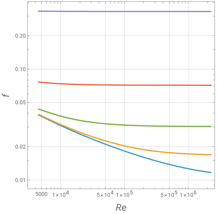
This generated a reference dataset of 2500 points.
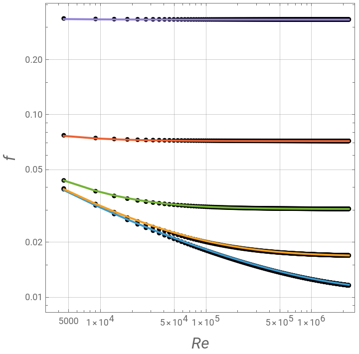
A- Haaland equation
1/sqrt(f) = -1.8 [ ((ε/D)/3.7 )^1.11 + 6.9/Re ]
log
10
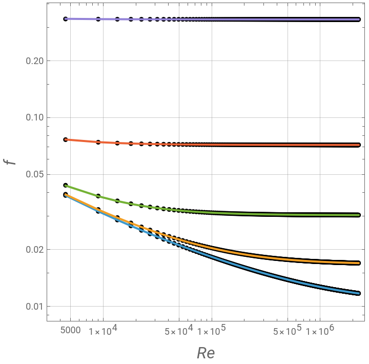
B- SGN correlation (see Ref. 1)This is a more complex explicit formulation depending on empirical Reynolds and roughness-dependent terms.Both models were evaluated at identical (Re, ε/D) points as the Colebrook-White dataset.

To quantify model accuracy, four statistical indicators were used:
1- Coefficient of determination ()
2
R
2- Nash-Sutcliffe Efficiency (NSE)
3- Mean Squared Error (MSE)
4- Root Mean Squared Error (RMSE)
The SGN formulation shows even lower numerical deviation, indicating a near-perfect reproduction of the reference dataset within machine precision limits.
Although both models yield ( = 1), this does not imply exact analytical equivalence. Instead, it indicates that:
Although both models yield (
2
R
• The deviations between models and Colebrook-White are extremely small
• Errors are below the resolution of standard floating-point correlation metrics
• Both correlations preserve the same functional trend across the turbulent flow regime
The SGN correlation shows marginally lower RMSE, suggesting slightly improved numerical fidelity compared to Haaland within the tested domain.
Therefore, RMSE and NSE provide more meaningful discrimination between models than in this case.
Therefore, RMSE and NSE provide more meaningful discrimination between models than
2
R
To summarize the findings, both explicit correlations provide highly accurate approximations of the Colebrook-White equation over a wide range of Reynolds numbers and roughness values. However:
• Haaland offers simplicity and robustness
• SGN provides slightly improved numerical accuracy
• Both are suitable substitutes for iterative Colebrook-White solutions in engineering applications
In[]:=
ColebrookWhite[Re_,epsOVERd_]:=f/.FindRoot[1/Sqrt[f]==-2Log10[(epsOVERd/(3.7))+(2.51/(ReSqrt[f]))],{f,0.02}]
In[]:=
LaunchKernels[]
Out[]=
KernelObject

In[]:=
relr={0.00005,0.0005,0.005,0.05,0.5};
In[]:=
dataCW=Flatten[Parallelize[Table[{i,relr[[j]],ColebrookWhite[i,relr[[j]]]},{i,4500,2250000,4500},{j,1,5,1}]],1];
In[]:=
Length@dataCW
Out[]=
2500
In[]:=
dataplot=.
In[]:=
dataplot[j_]:=Parallelize[Table[{i,ColebrookWhite[i,relr[[j]]]},{i,4500,2250000,4500}]]
p=ListLogLogPlotTable[dataplot[j],{j,1,5}],
Out[]=


Haaland[Re_,epsOVERd_]:=Module[{f},f=1/(-1.8*Log10[((epsOVERd)/3.7)^1.11+6.9/Re])^2;f]
In[]:=
dataHaaland=Table[{dataCW[[i]][[1]],Haaland[dataCW[[i]][[1]],dataCW[[i]][[2]]]},{i,1,2500}];
ShowListLogLogPlotdataHaaland,,p
Out[]=
In[]:=
R2[obs_List,sim_List]:=Correlation[obs,sim]^2
In[]:=
R2[(Transpose@dataplot)[[2]],(Transpose@dataHaaland)[[2]]]
Out[]=
1.
In[]:=
NSE[obs_List,sim_List]:=Module[{meanObs},meanObs=Mean[obs];1-Total[(obs-sim)^2]/Total[(obs-meanObs)^2]]
In[]:=
NSE[(Transpose@dataplot)[[2]],(Transpose@dataHaaland)[[2]]]
Out[]=
0.999993
MSE
mse=Mean[((Transpose@dataplot)[[2]]-(Transpose@dataHaaland)[[2]])^2]
Out[]=
1.07458×
-7
10
RMSE
rmse=Sqrt[mse]
Out[]=
0.000327808
In[]:=
SGN[Re_,epsOVERd_]:=Module[{s},s=0.1413*(epsOVERd)^0.9683*Re^0.9753+1.0392*Log[0.5238*Re^1.0474];1/(0.8811*Log[(0.4723*Re^0.9929)/(0.9574s^(0.9455s/(0.9291s+1.3)))])^2]
In[]:=
dataSGN=Table[{dataCW[[i]][[1]],SGN[dataCW[[i]][[1]],dataCW[[i]][[2]]]},{i,1,2500}];
ShowListLogLogPlotdataSGN,,p
Out[]=
In[]:=
R2[(Transpose@dataplot)[[2]],(Transpose@dataSGN)[[2]]]
Out[]=
1.
In[]:=
NSE[(Transpose@dataplot)[[2]],(Transpose@dataSGN)[[2]]]
Out[]=
1.
MSE
mse=Mean[((Transpose@dataplot)[[2]]-(Transpose@dataSGN)[[2]])^2]
Out[]=
1.96337×
-9
10
RMSE
rmse=Sqrt[mse]
Out[]=
0.00004431
References
References
[1] Roshan, S., Taleb Beydokhti, N., Afzali, S.H. et al. Estimating Pipe Friction Factors Using Machine Learning Approaches. Iran J Sci Technol Trans Civ Eng (2025). https://doi.org/10.1007/s40996-025-02008-9
CITE THIS NOTEBOOK
CITE THIS NOTEBOOK
Comparison of two explicit friction factor correlations using Colebrook-White as reference
by Housam Binous and Ahmed Bellagi
Wolfram Community, STAFF PICKS, May 14, 2026
https://community.wolfram.com/groups/-/m/t/3716240
by Housam Binous and Ahmed Bellagi
Wolfram Community, STAFF PICKS, May 14, 2026
https://community.wolfram.com/groups/-/m/t/3716240