ORIGINAL ARTICLE: Cahalan, R.F., Ajiquichí, P. & Yatáz, G. Solar Temperature Variations Computed from SORCE SIM Irradiances Observed During 2003–2020. Sol Phys 297, 16 (2022). https://doi.org/10.1007/s11207-021-01941-y
Article Abstract: NASA’s Solar Radiation and Climate Experiment (SORCE) Spectral Irradiance Monitor (SIM) instrument produced about 17 years of daily average Spectral Solar Irradiance (SSI) data for wavelengths 240 – 2416 nm. We choose a day of minimal solar activity, August 24, 2008 (2008-08-24), during the 2008 – 2009 minimum between Cycles 23 and 24, and compute the brightness temperature ) from that day’s solar spectral irradiance (). We consider small variations of T and SSI about these reference values, and derive linear and quadratic analytic approximations by Taylor expansion about the reference-day values. To determine the approximation accuracy, we compare to the exact brightness temperatures T computed from the Planck spectrum, by solving analytically for T, or equivalent root finding in Wolfram Mathematica. We find that the linear analytic approximation overestimates, while the quadratic underestimates, the exact result. This motivates the search for statistical “fit” models “in between” the two analytic models, with minimum root-mean-square-error, RMSE. We make this search using open-source statistical R software, determine coefficients for linear and quadratic fit models, and compare statistical with analytic RMSEs. When only linear analytic and fit models are compared, the fit model is superior at ultraviolet, visible, and near-infrared wavelengths. This again holds true when comparing only quadratic models. Quadratic is superior to linear for both analytic and statistical models, and statistical fits give the smallest RMSEs. Lastly, we use linear analytic and fit models to find an interpolating function in wavelength, useful when the SIM results need adjustment to another choice of wavelengths, to compare or extend to any other instrument. Advantages of the quadratic T over the exact T include ease of interpretation, and computational speed.
(
T
0
SSI
0
1. Harvard-Smithsonian Solar Spectral Irradiance (SSI) and Total Solar Irradiance (TSI)
1. Harvard-Smithsonian Solar Spectral Irradiance (SSI) and Total Solar Irradiance (TSI)
Solar irradiance is the Sun’s radiation integrated over the full solar disk, and expressed in SI units of power through a unit of area, . The commonly used term “full disk”, includes all of the Sun’s irradiance coming from the solar photosphere and temperature regimes at higher altitudes, including the chromosphere, transition region, and corona. In this notebook we display the “Solar Spectral Irradiance” or SSI, and it is integral, the “Total Solar Irradiance” or TSI. The TSI is the Sun’s irradiance integrated across all wavelengths at normal incidence to the top of the Earth’s atmosphere through a unit surface and at a range of 1 astronomical unit (AU). ( See ISO/DIS 21348, available at http://www.iso.org and for review at http://SpaceWx.com ). An Astronomical Unit or AU is a unit of length approximately equal to the annual mean distance between the Sun and Earth with a currently accepted value of (149 597 870 691 ±3) m (SI, 1998; DE405). The TSI was historically known as the “solar constant,” though it is not constant, but varies with the Sun’s magnetic activity. Variations in TSI have been monitored since measurements that began outside Earth’s atmosphere, initially in 1978 by NASA’s Earth Radiation Budget (ERB) instrument, an active cavity radiometer, that flew onboad the Nimbus 7 satellite. The Sun’s TSI and SSI are impacted by the highly variable weather on the Sun’s visible surface, the photosphere, especially at ultraviolet (UV) and shorter wavelengths. For simplicity of interpretation, we shall consider below an idealized SSI, typical of an imaginary “Quiet Sun” that lacks the violent weather events observed during a maximum of the 11-year sunspot cycle.
The solar irradiances used here were obtained from Gail Anderson of Phillips Lab, and were generated by Bob Kurucz at Harvard-Smithsonian. It is derived from a semi-empirical database that includes known atomic line transitions incorporated into a line-by-line code, depending on solar source (photosphere, chromosphere, corona). For details, contact:
Email: bob.kurucz%cfaku3.decnet@cfa.harvard.edu.
FAX: 617-495-7049, phone: 617-495-7429.
The original data was interpolated onto a regular 20 cm-1 wavenumber grid, from 60 cm-1 to almost 50,000 cm-1. These were stored in an ASCII dataset with each line giving the wavenumber in cm-1, and irradiance in W/(m2 cm-1) . We’ll see below how to transform between wavenumber and wavelength.
W/
2
cm
The solar irradiances used here were obtained from Gail Anderson of Phillips Lab, and were generated by Bob Kurucz at Harvard-Smithsonian. It is derived from a semi-empirical database that includes known atomic line transitions incorporated into a line-by-line code, depending on solar source (photosphere, chromosphere, corona). For details, contact:
Email: bob.kurucz%cfaku3.decnet@cfa.harvard.edu.
FAX: 617-495-7049, phone: 617-495-7429.
The original data was interpolated onto a regular 20 cm-1 wavenumber grid, from 60 cm-1 to almost 50,000 cm-1. These were stored in an ASCII dataset with each line giving the wavenumber in cm-1, and irradiance in W/(m2 cm-1) . We’ll see below how to transform between wavenumber and wavelength.
First turn of irrelevant warming messages, and read in the datafile:
In[]:=
Off[General::spelll];Directory[]
Out[]=
"C:\\Users\\TOSHIBA\\Desktop\\Math-12"
Adjust the argument of this command to point to the directory that contains the “SolarIrr.dat” file:
In[]:=
SetDirectory["C:/Users/TOSHIBA/Desktop/Math-12"]
Out[]=
C:\Users\TOSHIBA\Desktop\Math-12
Open the file to be read in the file, with each record a pair of numbers, the close the file:
In[]:=
fp=OpenRead["SolarIrr.dat"];
In[]:=
SSI=ReadList[fp,{Number,Number}];
In[]:=
Close[fp];
SSI now contains a list of spectral irradiance records, with each record consisting of a pair of numbers, {wavenumber, spectral irradiance}. We have that a=wavenumber and b=spectral irradiance, in this way the records are represented as : {{{a1},{a2}},{{a1},{b1}},...,{{an},{bn}}}.
In[]:=
bandcount=Length[SSI]
Out[]=
2496
So there are bandcount =2496 total records. In the List SSI we have to extract the list of wavenumbers, compute the min and max wavenumbers. The command transpose places the data in the form of a column and the first number is the wavenumber. In the Electromagnet Theory we know the relation between the wavenumber and wavelength (k=1/λ), and that is the reason about the wavenumber units cm-1
In[]:=
{minNu=Min[First[Transpose[SSI]]],maxNu=Max[First[Transpose[SSI]]]}
Out[]=
{60.,49960.}
The min and max of wavenumber is {60.0, 49960}.
We have an interval [minNu, maxNu], of n subintervals of width “bandwidth” (cm-1):
In[]:=
bandwidth=(maxNu-minNu)/(bandcount-1)
Out[]=
20.
Extract the spectral solar irradiance (SSI) values and get the maximum irradiance (W/(m2 cm-1))
In[]:=
maxIRR=Max[Last[Transpose[SSI]]]
Out[]=
0.0745
Extract the wavenumber at which the irradiance is maximum. Remember that for each wavenumber we have a spectral irradiance {wavenumber, spectral irradiance}
In[]:=
NumaxIRR=First[First[Cases[SSI,{_,maxIRR}]]]
Out[]=
11160.
2.0 Total Solar Irradiance (TSI) from Integrating Solar Spectral Irradiance (SSI)
2.0 Total Solar Irradiance (TSI) from Integrating Solar Spectral Irradiance (SSI)
Compute the TSI (total solar irradiance, formerly called “solar constant”) by adding all irradiances and multiplying by the bandwidth, assuming negligible energy outside the interval [minNu, maxNu], and also neglecting endpoint integration errors (that would be reduced by an improved integration method).
To obtain the Solar constant we use the integration method trapezoidal.
To obtain the Solar constant we use the integration method trapezoidal.
In[]:=
TSI=bandwidthPlus@@Last[Transpose[SSI]]
Out[]=
1366.91
Now compute TSI using “Integrate[Interpolation[data...]]”, setting the interpolation polynomial order k=4. The command Interpolation help us to find a function which helps us find a relationship between the data of wavenumber and spectral irradiance. We are going to integrate with respect wavenumber, and we use the minNu and maxNu as limits of integration.
In[]:=
TSIList=NIntegrate[Interpolation[SSI,InterpolationOrder4][x],{x,minNu,maxNu}]

Out[]=
1367.75
Apparently the endpoint error due to rectangular integration is small when we use the full range of wavenumber in SSI. However, just to be careful, let’s check whether the two constants are exactly equal:
In[]:=
Equal[TSI,TSIList]
Out[]=
False
So the two approximations to the Total Solar Irradiance, TSI, are not exactly equal. Below we use the Interpolation approach with InterpolationOrder > 4.
3.0 SimpleBandEnergy Function-Integrating over standard spectral intervals
3.0 SimpleBandEnergy Function-Integrating over standard spectral intervals
The wavelengths and band naming conventions employed below are taken from Table 1 of the draft ISO/DIS 21348, entitled “Space environment (natural and artificial) – Process for determining solar irradiances” (dated 2005-08-09). For convenience, we introduce SimpleBandEnergy, a function that is simple to apply to the wavelength bands defined in the draft ISO/DIS 21348. The function SimpleBandEnergy takes a input a par of wavelength in nm as units, in a list called nmLimits, computes it a corresponding pair of bandnumbers, and applies ListIntegrate to integrate SSI between those bandnumbers:
In[]:=
nmLimits[BNLimits_]:=10^7/(minNu+bandwidth(BNLimits-1));
In[]:=
BNLimits[nmLimits_]:=IntegerPart[(10^7/nmLimits-minNu)/bandwidth+1];
In[]:=
SimpleBandEnergy[nmLimits_]:=NIntegrate[Interpolation[Take[SSI,BNLimits[nmLimits]],InterpolationOrder4][x],{x,BNLimits[nmLimits][[1]],BNLimits[nmLimits][[2]]}];
To test these, first compute the max and min wavelength (nm), that correspond to the min and max bandnumbers, 1 and bandcount, respectively:
In[]:=
{maxNM,minNM}=nmLimits[{1,bandcount}]
Out[]=
{166667.,200.16}
The wavelength range is from 16667 NanoMeters(nm) to 200 nm. Similarly, test the inverse, to compute min and max bandnumbers from max and min wavelengths:
In[]:=
BNLimits[{maxNM,minNM}]
Out[]=
{1,2496}
Finally, test SimpleBandEnergy by checking to see if it gives the TSI when integrating over the full wavelength range:
In[]:=
Equal[SimpleBandEnergy[{maxNM,minNM}],TSIList]
Out[]=
False
Now define the wavelength pairs for bands taken from of the draft ISO/DIS 21348, from SpaceWx.com, with the larger wavelength listed first in each pair:
MUV={300,minNM};UVB={315,280};NUV={400,300};UVA={400,315};VIS={760,380};VISPurple={450,360};VISBlue={500,450};VISGreen={570,500};VISYellow={591,570};VISOrange={610,591};VISRed={760,610};IRA=NIR={1400,760};IRB=MIR={3000,1400};
These are only bands from the draft ISO/DIS 21348 that lie within {maxNM, minNM} of SSI. Note that in defining MUV, we replaced 200 nm by minNM=200.16 nm, introducing a small error. Now we compute the SimpleBandEnergy for each of these, and the associated SimplePercents:
In[]:=
SimpleBandEnergies={MUVBandEnergy=SimpleBandEnergy[MUV],UVBBandEnergy=SimpleBandEnergy[UVB],NUVBandEnergy=SimpleBandEnergy[NUV],UVABandEnergy=SimpleBandEnergy[UVA],VISBandEnergy=SimpleBandEnergy[VIS],PurpleBandEnergy=SimpleBandEnergy[VISPurple],BlueBandEnergy=SimpleBandEnergy[VISBlue],GreenBandEnergy=SimpleBandEnergy[VISGreen],YellowBandEnergy=SimpleBandEnergy[VISYellow],OrangeBandEnergy=SimpleBandEnergy[VISOrange],RedBandEnergy=SimpleBandEnergy[VISRed],IRABandEnergy=NIRBandEnergy=SimpleBandEnergy[IRA],IRBBandEnergy=MIRBandEnergy=SimpleBandEnergy[IRB]};
In[]:=
SimplePercents=100*SimpleBandEnergies/TSIList;
In[]:=
SIMEnergyPercent=100*SimpleBandEnergy[{2400,minNM}]/TSIList;
When adding these percents, care must be taken to account for the overlaps between some of these bands. For example, UVA overlaps VIS, and VISPurple overlaps both UVA and VIS. Also, SimpleBandEnergy can give nonsense when applied to wavelengths outside of {maxNM, minNM}, to bands that are too narrow, or to wavelengths in the wrong order. An example of the latter is SimpleBandEnergy[{minNM, maxNM}] which generates an error message.
4.0 Plots of SSI vs Wavenumber, and vs Wavelength
4.0 Plots of SSI vs Wavenumber, and vs Wavelength
Now let’s take a closer look at the shape of this function SSI, that we’ve been integrating, and afterwards we’ll compare SSI to a smooth blackbody spectrum having the same total energy. The Spectral Solar Irradiance SSI may be plotted as a function of wavenumber as follows:
In[]:=
labelticks[range_]:=MapIndexed[Which[OddQ[First[#2]],{#1,#1,{0.030,0}},EvenQ[First[#2]],{#1,"",{0.015,0}}]&,range]
In[]:=
$DefaultFont={"Times-Bold",14};
In[]:=
xmarks=Range[0,30000,5000];
In[]:=
ymarks=Range[0,0.1,0.01];
In[]:=
bottom=top=labelticks[xmarks];
In[]:=
left=right=labelticks[ymarks];
This graphic show how is the variation of the Irradiance in different wavenumber.
In[]:=
gdata=ListPlot[SSI,PlotRange{{0,30000},{0,0.1}},JoinedTrue,FrameTrue,FrameLabel{"Wavenumber (\!\(\*SuperscriptBox[\(cm\), \(-1\)]\))","Irradiance(W/(\!\(\*SuperscriptBox[\(m\), \(2\)]\)*\!\(\*SuperscriptBox[\(cm\), \(-1\)]\)))"},PlotLabelStyle["TOA Spectral Solar Irradiance"],FrameTicks{bottom,left,top,right},PlotStyle{RGBColor[1,0,0]}]
Out[]=
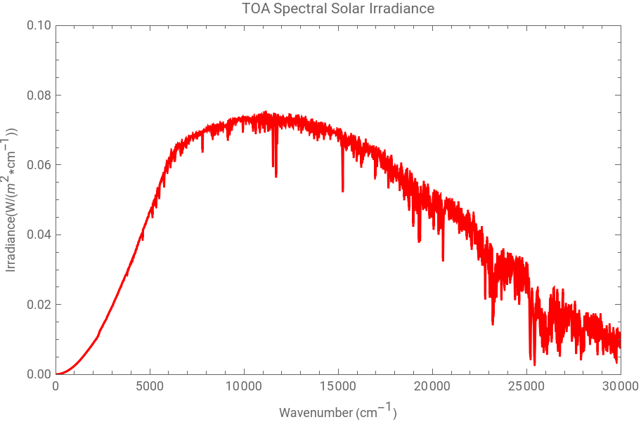
Note, as mentioned before, that the peak in SSI is near wavenumber 10000 (actually at NumaxIRR=11160) corresponding to 1000 nm. Below we show that changing variables, and multiplying by the Jacobian |dNu/dNM|, gives a spectral distribution that peaks close to 500 nm. The most obvious absorption lines in the above plot are from doubly-ionized Calcium (Ca-II)--a triplet just below 12000 , and a doublet just above 25000 . One can also identify the first few lines in teh hydrogen Balmer series at. The Balmer series is just applied for the hydrogen atom, and the equation is this: 1/λ = (1/B)*(1-4/) where B [cm] is an experimental constant.
To learn more about Balmer Series, this is a good reference : http://www.phys.utk.edu/labs/modphys/BalmerSeries.pdf
-1
cm
-1
cm
2
n
To learn more about Balmer Series, this is a good reference : http://www.phys.utk.edu/labs/modphys/BalmerSeries.pdf
In[]:=
B:=3.6457879*10^(-5)
Now we are going to obtain the four Balmer wavenumber (cm-1) for the Hydrogen atom:
In the Electromagnetic Theory we know the relation between wavenumber and wavelength (k=1/λ), using this relation we can obtain the Balmer wavelength ( cm).
Now we have to convert from cm to nm.
Using the draft ISO/DIS 21348, these are all in the Visible, the First in the Red, The second in the Blue, and the last two in the Purple and NUV. Individual photon energies for these transitions are given by: E=hc/λ, where “h” is Planck’s constant, c is speed of the light in vacuum and λ es wavelength. Expressing hc=1239.84 electronVolt*nm, now we can calculate the Balmer energy.
So an electron that drops from the n=3 to the n=2 bound state releases a photon carrying Energy =HEnergy[[3]]-HEnergy[[2]]={-1.51111 eV} - {-3.4 eV}=1.89 eV. Similarly, and electron that drops from n=2 to the Hydrogen ground state at n=1 releases a photon with Energy =HEnergy[[2]]- HEnergy[[1] ]={-3.4 eV} - {-13.6 eV}=10.2 eV.
With Albert Einstein’s Theory for the photoelectric effect, where a photon has a energy proportional to its frequency, Bohr postulated the existence of energy levels in the atom. He assumed that the energy associated with the photons of light were the result of transition in the atom from one level to another.
With Albert Einstein’s Theory for the photoelectric effect, where a photon has a energy proportional to its frequency, Bohr postulated the existence of energy levels in the atom. He assumed that the energy associated with the photons of light were the result of transition in the atom from one level to another.
We can obtain the equal result using the energy of the electron that drops from n =2 to n=1.
The corresponding emission line in the solar spectrum at 121.553 nm is called the “Lyman Alpha” line. The wavenumber of Lyman Alpha with unit cm-1 is:
We cannot display this emission line, because our data only extend to maxNu=49960. Before comparing the spectrum to a Blackbody, let’s first display the spectrum as a function of wavelength , in nm. To do that, we first change the list of wavenumbers in SSI into a list of NanoMeters (nm, also NM):
We must also make sure that the energy integrals over any band are invariant when changing variables, which is done by multiplying SSI by the Jacobian of the transformation. In this case the variable change is: Nu=10^7 /NM and the Jacobian is | dNu/dNM|=10^7/NM^2 =Nu^2/10^7
Combine the wavelengths and irradiances into a list of pairs {NanoMeters, SSINanoMeters}. We know that the irradiance is in SSI NanoMeters
Get the maximum irradiance in SSINanoMeters W/ (m2 nm)
Extract the wavelength in nm at which the irradiance is maximum:
Finally, plot SSINM in the same way as we previously plotted SSI:
As promised, this peaks near 500 nm, actually about 451 nm. Here the Calcium II doublet appears just below 400 nm, the Hydrogen Balmer lines appear at { 434 , 486 , 656 } nm with photon energy { 2.86 , 2.55 , 1.89 } eV, and the Calcium II triplet appears nears 833 nm. The next section compares SSI and SSINM with a smooth analytic Blackbody spectrum.
5.0 BlackBody Irradiance for T=5780 K
5.0 BlackBody Irradiance for T=5780 K
Let’s compare the above data with irradiance from a blackbody at T = 5780 K, where T is chosen to give approximately the same TSI. To define the blackbody spectrum, we need to specify the Stefan-Boltzmann constant (sigma with units W/(m^2 *K^4)), the Sun’s radius (RS), and surface are (areaS), and the Sun-Earth distance (dE). For later use, we also give the Earth’s radius (RE), surface are (areaE) and albedo (albedoE). We are going to use Metric-Kilogram-Second units:
The Stefan-Boltzmann law describes the power radiates from a black body in terms of its temperature. The total energy radiated per unit surface area of a black body is directly proportional to the fourth power of the black body’s temperature. So, we are going to calculate the energy radiate for the Sun, suing TS=5780 Kelvin. Also this is know as “effective radiative temperature” of the Sun:
Assuming that the Earth is in thermal equilibrium with the fraction of solar energy that it absorbs, we show below that the effective radiative temperatures of the Earth is 255 Kelvin, so that the Earth’s total output power, in Watts is:
For more information about the follows calculus, you can read this document in this page: http://www.iki.rssi.ru/asp/pub_sha1/Sharch06.pdf
The Planck blackbody radiance distribution in terms of frequency (Hz) and temperature (K) is:
For this constant, remember that hc=1239.84 eV*nm and k_B=8.617333*10^(-5)eV/K
It is necessary to convert from K*nm to K*cm
The maximum radiance is given as a function of temperature by:
This is the equation of wavenumber where is the maximum radiance as a function of temperature (v_peack)
For T= 5780 K, these have the values:
The blackbody maximum occurs at a wavenumber only slightly that where the data is maximum, which was determined above and is repeated for convenience here:
The analogous formulas in terms of the wavelength λ(nm) are:
The solid angle subtended by the Sun at Earth’s distance can be computed as the total solid angle of a sphere of radius dE centered on the Earth, 4*Pi, times the fractional are the Sun intercepts on the sphere, namely Pi*(R_s)^2/(4*Pi*(dE)^2)=(R_s/dE)^2/4, so that:
Then, the maximum Solar Irradiance at T=2780 k is:
The agreement of maxIRR and with the BlackBody is particularly close, while maxIRRNM is well above the blackbody value from SUNangle*Bλmax, as will be evident in the camparison plots below. The Blackbody Irradiance as a function of wavenumber for T=5780 K is plotted as follows:
To facilitate comparison, this T=5780 K blackbody plot may be superimposed on the data:
The plot shows the close agreement of the data peak, at maxIRR with the peak of the blackbody curve, at SUNangle*Bmax[5780].
As an alternative to plotting solar irradiance vs wavenumber, let us now plot blackbody irradiance vs wavelength λ, for T=5780 K, as follows:
As an alternative to plotting solar irradiance vs wavenumber, let us now plot blackbody irradiance vs wavelength λ, for T=5780 K, as follows:
Again, as with the SSI data, changing from wavenumber to wavelength moves the peak from about 1 Micron to about 0.5 Micron. As donde above in wavenumber, to facilitate comparison with the data, the above T=5780 K blackbody plot versus wavelength, maybe superimposed on the plot of the SSINM data:
This plot shows a clear discrepancy between the data and the Blackbody. At the peak of the Blackbody curve, at SUNangle Bmax[5780], the curve lies well below the peak of the data, at NMmaxIRR. This discrepancy, about 20% at the data peak, is compensated by a reverse discrepancy below about 400 nm, where the blackbody significantly exceeds the data. On the other hand, above the Hydrogen Balmer line at 676 nm, and continuing into the NIR and MIR, the Blackbody appears to agree quite well with the data. However, a slight deficiency is seen in the Blackbody curve near 1600 nm = 1.6 mm. That discrepancy becomes much more evident when the plot is transformed to “equivalent blackbody temperature” as in the next section.
We are going to open a new database
For this database, the first number is wavelength (nm) and the second is the Irradiance.
In this moment we are going to compare the result of this new database “SolarIrrSORCE” with the result of Blackbody.
6.0 Plots of SSI vs Equivalent Blackbody Temperature (Teq)
6.0 Plots of SSI vs Equivalent Blackbody Temperature (Teq)
One way to think of discrepancies between observed SSI and blackbody curve is in terms of the “equivalent brightness temperature”, Teq, which is the Blackbody temperature for which a Blackbody curve would through the data at a given wavelength. For example, when λ=NMmaxIRR, near 450 nm, the value of Teq that gives the observed SSI is slightly above 6000 K.
This is the wavelength where we have the maximum irradiance:
The Solar Spectral Irradiance maximum (Blackbody), at wavelength=450 nm and T=5780 K is:
The Solar Spectral Irradiance with at wavelength= 450 nm using the data SSI in nanometers (SSINM). Remember that SSINM is a list of pairs {NanoMeters, SSINanoMeters}, this is: SSINM =Transpose[{NanoMeters, SSINanoMeters}]
The unit of SSIλ is [W/(m^2 nm)]
In this moment we are going to found the temperature in SSI, where SSIλ and SUNangle Bλ are equal.
The value of Teq that gives the observed SSI is slightly above 6000 K.
To compute Teq for a range of wavelengths, it is convenient to first define an “interpolating function” that allows SSINM to be evaluated at an arbitrary wavelength. We then apply FindRoot to a convenient list of wavelengths, and finally search the list to find the extrema of “Teq”.
The first numbers are temperatures: 3984.45 K and 6436.06 K, and the last numbers are wavelengths: 200 nm and 1630 nm
Finally, we plot TeqLsit in the same way as we previously plotted SSINM:
Another feature that becomes clear in the “Teq” plot is that NIR and MIR absorption lines become more evident. Several lines above 1600 nm now stand out clearly, which were nearly invisible in the irradiance plots.
Let’s try to extend the list and the plot of Teq values beyond 300 nm , into the FIR (40,000 nm a 350000 nm):
The first numbers are temperatures: 3984.45 K and 7951.45 K, and the last numbers are wavelengths: 200 nm and 154 820 nm.
The maximum Teq of nearly 8000 K, found in LongTeqList in the FIR near 155 microns (155, 000 nm), disagrees with measurements. There should be a minimum near 70 cm^(-1)=142 ,microns, ssociated with the minimum in the solar temperature in the transition zone between the photosphere and the corona. The following plot reveals the origin of this disagreement:
We are going to plot the data of LongTeqList
Though the Teq appears to be approaching and FIR minimum up to about 70 000 nm. The increasing bumpiness seen at wavelengths above 70,000 micrometers indicates problems with the interpolating function, SSIλ, at the longer wavelengths, where the wavelength spacing becomes large.
The spacing between the longest 2 wavelengths is more than 40,000 nm
The spacing between the first 2 wavelengths is less than 0.1 nm.
So care must be taken in using this data beyond about 3000 nm, into the FIR, despite the fact that values of SSIλ are provided for wavelengths up to 167,000 nm. We have that SSISM =ReadList[fp, {Number, Number}]. The SSISIM is a new database, SolarIrradiance
The first numbers are temperatures: 179.752 K and 6560.64 K, and the last numbers are wavelengths: 246 nm and 1700 nm
In this moment, we compare the two graphics, gTeqSolar (SSISM)and gTeqSolarSIM.
7.0 Integrals Compared: T=5780 K BlackBody vs Solar Data
7.0 Integrals Compared: T=5780 K BlackBody vs Solar Data
The Total Solar Irradiance (TSI) that corresponds to the T=5780 K blackbody curve, assuming negligible energy outside the interval [minNu, maxNu], is obtained by integration as follows:
This is the minimum wavenumber from the data SSI
This is the maximum wavenumber from the data SSI
The Total Solar Irradiance (units: W/m^2) using the minimum and maximum wavenumber is:
This is the integral over the data, which is repeated for convenience here.
The energy in the blackbody curve which is below and above the interval [minNu, maxNu] is :
Thus the blackbody estimate of the missing energy is about 2 W/m^2 out of about 1367 W/m^2, from wavenumbers above maxNu, or wavelengths below about 200 nm. In percentage terms, the missing energy is about:
So we estimate that the missing energy is 0.15% of the TSI, at wavenumbers above maxNu, or wavelengths below minNM, shorter than the MUV. As we will see below, the blackbody tends to overstimate the energy at UV wavelengths, when compared to the “Quiet Sun” so the above PercentMissing blackbody estimate is likely an overestimate of the energy coming from wavelengths shorter than 200 nm, at least when the Sun is not too active. Previously we defined a function called SimpleBandEnergy, that takes as input a pair of wavelengths in nm, in a list called nmLimits, computes from it a corresponding pair of bandnumbers, and applies ListIntegrate to integrate the data-derived solar spectrum, SSI, between those bandnumbers. To facilitate comparison of the data-based ListIntegrals with Integrals over the analytic 5780 K BlackBody spectrum, we now define an analogous function that applies NIntegrate to the Blackbody spectrum: .
8.0 Earth 255 K BlackBody compared to Solar BlackBody*(1-albedoE)/4
8.0 Earth 255 K BlackBody compared to Solar BlackBody*(1-albedoE)/4
The energy emitted by the Sun in the Earth per unit area is:
The energy reflected by the Earth per unit area is:
The solar energy absorbed by the Earth per unit area is:
where the factor of (1/4) is the ratio of the total area of the Earth, all of which emits radiations towards space, to its cross-sectional area, which absorbs the incoming solar radiation. [Note that the factor (1/4) applies only for the global average energy balance, typical of mid-latitudes. At low-latitudes, more solar energy is absorbed, because Earth areas tend to be more perpendicular to the Sun’s rays, while at high latitudes, areas are more oblique to incoming rays, so tend to absorb less.] The total infrared energy emitted from the Earth is the Earth’s area times sigma*(Teff)^4, where Teff is the effective radiative temperature of the Earth. So in equilibrium we must have that,
the temperature (K) is:
the temperature (K) is:
To compare the spectrum of Earth’s emitted radiation with the absorbed Solar Radiation, per unit area, we multiply the incoming Solar spectrum by (1-albedoE)/4, and multiply the Earth-emitted radiance B(Teff) by Pi to account for the angular integration over the outgoing hemisphere. This gives:
The peak of the Earth’s blackbody radiation curve is at:
To check that the integral of this Earth curve balances the SolarIn:
If we expand the region from the origin to wavenumber 2000 ( cm^-1), the the Earth irradiance becomes more obvious:
The peak of this curve occurs at wavenumber 500, corresponding to 20 Microns. As we have already seen with SSI, when we plot Earth’s spectral irradiance distribution versus wavelength, the peak will occur at about half the above wavelength, or 10 Microns.
The maximum Earth blackbody irradiance is:
The maximum Earth blackbody irradiance is:
Of course, the actual outgoing Earth radiation is different from a Blackbody because of absorption and emission processes, especially due to H20, C02, CH4, and 03.
Let us now redo the above plots in terms of wavelength. Then the vertical scales for Sun and Earth, respectively, are set by:
So we first choose 0.4 vertical scale to show the full solar blackbody spectrum, then change the vertical scale to 0.015 when zooming in on longer wavelengths to get a better view of the Earth equivalent blackbody spectrum.
As with the previous wavenumber plots, these 2 wavelength curves enclose the same area. Here the qualitative shapes of the Sun and Earth curves have reversed, with the Solar curve peaking at low values of wavelength, and the terrestrial curve stretching to longer wavelengths. Let’s now focus the plot on the longer terrestrial wavelengths:
Note that the “crossover” wavelength, where the spectral solar irradiance, the SSI, is first exceeded by the Earth-emitted irradiance, EEI, occurs just below 5000 nm. This wavelength is computed explicitly as follows:
So the crossover is at 4650 nm. Much shorter wavelengths, commonly called “shortwave” in Earth science, are predominantly of solar origin, while the much longer wavelengths, “longwave” in Earth science, mainly originate from Earth emission. Photons near crossover are of mixed origin. Note that 4.65um is the global average crossover, typical of mid-latitudes. At low latitudes there is an excess of incoming solar over outgoing longwave radiation, so that the crossover occurs at longer wavelengths, and conversely at high latitudes. Note that the crossover wavelength is not changed by the transformation between wavelength and wavenumber, because the Jacobian cancels out, so we find the same result for the wavenumber-equivalent crossover wavelength:
9.0 Earth 255 K BlackBody compared to observered Earth Emitted Irradiance (EEI):
9.0 Earth 255 K BlackBody compared to observered Earth Emitted Irradiance (EEI):
Finally, let’s compare the above idealized Earth-emitted blackbody, π Ba[v,Teff] or the equivalent π Bλ[λ,Teff], with a more realistic spectrum based on Earth observations. As with the Sun’s SSI, which as we’ve seen displays dramatic lines from absorption (or emission) by atoms in the Sun’s atmosphere, similarly, the real Earth-emitted Irradiance (EEI) shows deviations from the smooth blackbody curve, from absorption by molecules and aerosols in Earth’s atmosphere. To obtain something equivalent to the Sun’s SSI, for the Earth, the observed EEI, we must rely upon measurements made during two space missions -- NASA’s IRIS instrument, which operated for 9 months in 1970, and JAXA’s IMG, that collected data during 10 months in 1997. Both were interferometers, operated as infrared imaging spectrometers. Here we look only at the IRIS data. For comparison with IMG, see Harries et al (2003). Earth’s emission spectrum is strongly impacted by highly variable liquid and ice clouds, that vary with Earth’s variable weather, both temporally and geographically, and by the surface properties that are exposed beneath any cloud-free regions. Thus for simplicity of interpretation, we shall choose a large region of the central Pacific Ocean, and select only data that passes a “cloud-free threshold” test. The idealized “cloud-free Earth” is analogous to the “Quiet Sun” that lacks sunspots and associated weather on the Sun.
10.0 Lifetime of the Sun
10.0 Lifetime of the Sun
We defined the value of astronomical unit (AU) using the WolframAlpha data:
The Astronomical Unit (m)
This is the mass (kg) of the Sun obtained in Wolfram Mathematica
This is the speed of light obtained using WolframMathematica
The speed of the light (m/s):
The energy (J) of the Sun:
A list of TSI to calculate the lifetime of the Sun {{TSI, year}}:
We obtain a list of Total Solar Irradiance (W/m^2) for different years
The unit of luminosity is W=J/s:
For the calculus of the lifetime of the Sun, we use this equation, lifetime=Energy/Luminosity, where second is the unit of lifetime in the first calculus
Convert lifetime from second to years
Convert lifetime from years to billions years
CITE THIS NOTEBOOK
CITE THIS NOTEBOOK
Solar Temperature Variations Computed from SORCE SIM Irradiances Observed During 2003 – 2020
by Robert Cahalan, Paulino Ajiquichí, Gaspar Yatáz
Wolfram Community, STAFF PICKS, December 17, 2023
https://community.wolfram.com/groups/-/m/t/3085770
by Robert Cahalan, Paulino Ajiquichí, Gaspar Yatáz
Wolfram Community, STAFF PICKS, December 17, 2023
https://community.wolfram.com/groups/-/m/t/3085770