ORIGINAL ARTICLE: Pintér JD, Kampas FJ, Castillo I. Finding the Conjectured Sequence of Largest Small n-Polygons by Numerical Optimization. Mathematical and Computational Applications. 2022; 27(3): 42. DOI: https://doi.org/10.3390/mca27030042
Article Abstract: 𝐿𝑆𝑃(𝑛), the largest small polygon with 𝑛 vertices, is a polygon with a unit diameter that has a maximal area of 𝐴(𝑛). It is known that for all odd values , 𝐿𝑆𝑃(𝑛) is a regular 𝑛-polygon; however, this statement is not valid even for values of 𝑛. Finding the polygon 𝐿𝑆𝑃(𝑛) and 𝐴(𝑛) for even values has been a long-standing challenge. In this work, we developed high-precision numerical solution estimates of 𝐴(𝑛) for even values , using the Mathematica model development environment and the IPOPT local nonlinear optimization solver engine. First, we present a revised (tightened) LSP model that greatly assists in the efficient numerical solution of the model-class considered. This is followed by results for an illustrative sequence of even values of 𝑛, up to . Most of the earlier research addressed special cases up to , while others obtained numerical optimization results for a range of values from . The results obtained were used to provide regression model-based estimates of the optimal area sequence {𝐴(𝑛)}, for even values 𝑛 of interest, thereby essentially solving the LSP model-class numerically, with demonstrably high precision.
𝑛≥3
𝑛≥6
𝑛≥4
𝑛≤1000
𝑛≤20
6≤𝑛≤100
Introduction
Introduction
The goal of the calculation is to find the n-sided polygon with the largest area, with all the diagonals having length 1 or less.
Parametric IPOPT Minimize Code
Parametric IPOPT Minimize Code
SetUp
SetUp
The n vertices are described using polar coordinates, with the nth vertex at the origin, so that r[n] = θ[n] = 0.
The area of the polygon is calculated by dividing the polygon into triangles by running lines from the last vertex to the other vertices. Here is an example for a 7 sided polygon
The area of the polygon is calculated by dividing the polygon into triangles by running lines from the last vertex to the other vertices. Here is an example for a 7 sided polygon
In[]:=
exampleN=7;
In[]:=
examplePts=Table{0,1}+RotationMatrix.CirclePoints[exampleN][[i]],{i,exampleN}//N;
π
exampleN
In[]:=
exampleLines=Table[Line[{examplePts[[exampleN]],examplePts[[i]]}],{i,1,exampleN}];
In[]:=
Show[Region@RegionBoundary[Polygon[examplePts]],Table[Graphics@{PointSize[Large],Point[examplePts[[i]]]},{i,exampleN}],Graphics/@{Green,exampleLines},ImageSize->Small,Axes->True]
Out[]=
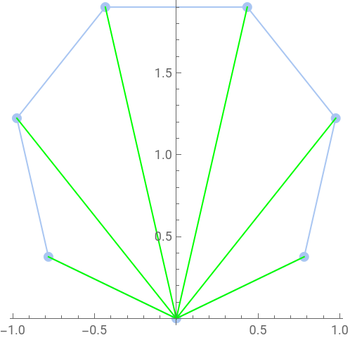
The area of each triangle can be calculated using the SASTriangle function.
In[]:=
Area@SASTriangle[r[i],θ[i+1]-θ[i],r[i+1]]
Out[]=
1
2
Since the angle between any two lines is always less than π/2, we can formulated the total area using the following formula, where n is the number of vertices.
In[]:=
obj[n_]:=Sum[r[i]*r[i+1]*Sin[θ[i+1]-θ[i]],{i,n-1}]
1
2
Next we need to calculate the length of the diagonals. We define a formula for the square of the distance between two points and use it to calculate the square of the length of the diagonals.
In[]:=
distSqr[pt1_,pt2_]:=(pt1-pt2).(pt1-pt2)
In[]:=
distSqr[r[i]{Cos[θ[i]],Sin[θ[i]]},r[j]{Cos[θ[j]],Sin[θ[j]]}]//FullSimplify
Out[]=
2
r[i]
2
r[j]
This is a plot of all the diagonals of the example.
In[]:=
exampleDiags=Flatten@Table[Line[{examplePts[[i]],examplePts[[j]]}],{i,exampleN-1},{j,i+1,exampleN}];
In[]:=
Show[Graphics@exampleDiags,ImageSize->Small,Frame->True]
Out[]=
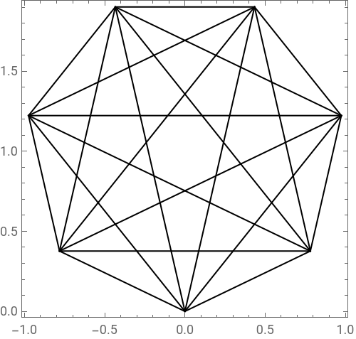
Since the length of the diagonals from the point at the origin to the other points is equal to the variable r[i] for the other points, the diagonal constraints from r[n] to the other points can be eliminated from the diagonal constraints by restricting the value of r[i] for the other points to be between 0 and 1.
In[]:=
exampleDiagsO=Flatten@Table[Line[{examplePts[[i]],examplePts[[j]]}],{i,exampleN-2},{j,i+1,exampleN-1}];
In[]:=
Show[Graphics@exampleDiagsO,Table[Graphics@{PointSize[Medium],Point[examplePts[[i]]]},{i,exampleN}],Frame->True]
Out[]=
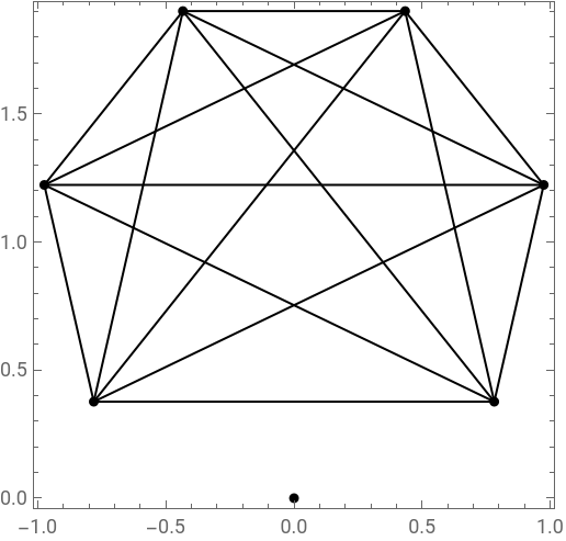
Since the constraint is that the length of the diagonals be <= 1, we can constrain the square of the length to be <= 1, where n is the number of vertices.
In[]:=
consDiag[n_]:=Flatten@Table[+-2r[i]*r[j]*Cos[θ[i]-θ[j]]≤1,{i,n-2},{j,i+1,n-1}]
2
r[i]
2
r[j]
The bounds of the variables are 0 <= r[i] <= 1 except for r[n] which is 0 <= r[n] <= 0 and 0 <= θ[i] <= π except for θ[n] : π <= θ[n] <= π
In[]:=
vwb[n_]:=Join[Table[{θ[i],0,π},{i,n-1}],{{θ[n],π,π}},Table[{r[i],0,1},{i,n-1}],{{r[n],0,0}}]
For even n, we add the following inequality constraint on the difference of consecutive values of θ[i]
In[]:=
consEven[n_]:=Table[θ[i+1]-θ[i]≥π/n,{i,n-2}]
For odd n, we add the following inequality constraint on the difference of consecutive values of θ[i]
In[]:=
consOdd[n_]:=Tableθ[i+1]-θ[i]==,{i,n-2}
π
n
The optimization is done with IPOPT, through a built-in Mathematica interface. It requires starting values for the search.
The starting value for θ[i] is π*i/n and the starting value for r[i] is 1 except for r[n] which has a starting value of 0.
The starting value for θ[i] is π*i/n and the starting value for r[i] is 1 except for r[n] which has a starting value of 0.
In[]:=
start[n_]:=Join[π*Range[n]/n,Table[1,n-1],{0}]
In order to show the diagonals with length near 1, the following function is defined.
In[]:=
bigDiags[n_,sln_]:=Select[Flatten[Table[{Sqrt[+-2r[i]*r[j]*Cos[θ[i]-θ[j]]],Line[{{r[i]*Cos[θ[i]],r[i]*Sin[θ[i]]},{r[j]*Cos[θ[j]],r[j]*Sin[θ[j]]}}]},{i,n-1},{j,i+1,n}]/.sln[[2]],1],#[[1]]>=0.999&]
2
r[i]
2
r[j]
The following two functions perform the optimization for an even number of vertices and an odd number of vertices, respectively and plot the polygon, with the diagonals with length >= 0.999 shown in red.
optEven[n_]:=Block[{sln=iMin[-obj[n],Join[consDiag[n],consEven[n],{θ[n/2]π/2}],vwb[n],{start[n]}],sides,diags},lns=Table[Line[{{r[i]*Cos[θ[i]],r[i]*Sin[θ[i]]},{r[i+1]*Cos[θ[i+1]],r[i+1]*Sin[θ[i+1]]}}],{i,n-1}]/.sln〚2〛;sides=Join[lns,{Line[{{0,0},{r[1]*Cos[θ[1]],r[1]*Sin[θ[1]]}}]}]/.sln〚2〛;diags=bigDiags[n,sln];Print@Show[Graphics/@sides,Graphics/@{Red,diags[[All,2]]},ImageSize->Small];{-sln[[1]],sln[[2]]}]
optOdd[n_]:=Block[{sln=iMin[-obj[n],Join[consDiag[n],consOdd[n],{θ[1]+θ[n-1]π}],vwb[n],{start[n]}],sides,diags},lns=Table[Line[{{r[i]*Cos[θ[i]],r[i]*Sin[θ[i]]},{r[i+1]*Cos[θ[i+1]],r[i+1]*Sin[θ[i+1]]}}],{i,n-1}]/.sln〚2〛;sides=Join[lns,{Line[{{0,0},{r[1]*Cos[θ[1]],r[1]*Sin[θ[1]]}}]}]/.sln〚2〛;diags=bigDiags[n,sln];Print@Show[Graphics@sides,Graphics/@{Red,diags[[All,2]]},ImageSize->Small];{-sln[[1]],sln[[2]]}]
Test
Test
CITE THIS NOTEBOOK
CITE THIS NOTEBOOK
Finding the Conjectured Sequence of Largest Small n-Polygons by Numerical Optimization
by János D. Pintér, Frank J. Kampas, and Ignacio Castillo
Wolfram Community, STAFF PICKS, November 9, 2023
https://community.wolfram.com/groups/-/m/t/3062624
by János D. Pintér, Frank J. Kampas, and Ignacio Castillo
Wolfram Community, STAFF PICKS, November 9, 2023
https://community.wolfram.com/groups/-/m/t/3062624