Doehlert Design for Wet Pelletization in High Shear Mixer
Authors: Housam Binous and Ahmed Bellagi
Doehlert Design for Wet Pelletization in High Shear Mixer
Authors: Housam Binous and Ahmed Bellagi
Authors: Housam Binous and Ahmed Bellagi
Three factors interfere in the determination of pellet mean size . These are the impeller speed, the binding solution and the pelletization time . We use experimental design (Doehlert design) to predict pellet mean size versus the three factors . We determine the quadratic model by multi - linear regression of the mean particle size . In addition, contour plots of the mean size versus impeller speed and the pelletization time for different biding solutions are given .
Acknowledgement :
1- This problem was presented by Lewis G. A., D. Mathieu and R. Phan-Than-Luu, Pharmaceutical Experimental Design, Drugs and the Pharmaceutical Sciences, Vol 92, 1999, Marcel Dekker, New York.
2- We also used the ideas for Placing a ContourPlot under a Plot3D from: https://community.wolfram.com/groups/-/m/t/1148582
In[]:=
Off[General::"spell1"]
Three Factors:
1/ Impeller Speed (rpm)=
Associated variable: X1, Lower level: 250, Upper level: 400
2/ Amount of binding solution (%)=
Associated variable: X2, Lower level: 60 Upper level: 70
3/ Pelletization time (min)=
Associated variable: X3, Lower level: 5 Upper level: 20
One Response:
Mean size of pellets (mm)
Plan and Experimental Results
In[]:=
TableForm[{{N°,X1,X2,X3,Speed,Solution,time,Size},{1,0,0,0,325,65.0,12.5,1594},{2,1,0,0,400,65.0,12.5,1398},{3,0.5,0.866,0,362,69.3,12.5,1352},{4,-0.5,0.866,0,288,69.3,12.5,1466},{5,-1,0,0,250,65.0,12.5,1750},{6,-0.5,-0.866,0,288,60.7,12.5,1064},{7,0.5,-0.866,0,362,60.7,12.5,1337},{8,0.5,0.289,0.816,362,66.4,18.6,1533},{9,-0.5,0.289,0.816,288,66.4,18.6,1617},{10,0,-0.577,0.816,325,62.1,18.6,1332},{11,0.5,-0.289,-0.816,326,63.6,6.4,1409},{12,-0.5,-0.289,-0.816,288,63.6,6.4,1560},{13,0,0.577,-0.816,325,68.9,6.4,1431}}]
Out[]//TableForm=
N° | X1 | X2 | X3 | Speed | Solution | time | Size |
1 | 0 | 0 | 0 | 325 | 65. | 12.5 | 1594 |
2 | 1 | 0 | 0 | 400 | 65. | 12.5 | 1398 |
3 | 0.5 | 0.866 | 0 | 362 | 69.3 | 12.5 | 1352 |
4 | -0.5 | 0.866 | 0 | 288 | 69.3 | 12.5 | 1466 |
5 | -1 | 0 | 0 | 250 | 65. | 12.5 | 1750 |
6 | -0.5 | -0.866 | 0 | 288 | 60.7 | 12.5 | 1064 |
7 | 0.5 | -0.866 | 0 | 362 | 60.7 | 12.5 | 1337 |
8 | 0.5 | 0.289 | 0.816 | 362 | 66.4 | 18.6 | 1533 |
9 | -0.5 | 0.289 | 0.816 | 288 | 66.4 | 18.6 | 1617 |
10 | 0 | -0.577 | 0.816 | 325 | 62.1 | 18.6 | 1332 |
11 | 0.5 | -0.289 | -0.816 | 326 | 63.6 | 6.4 | 1409 |
12 | -0.5 | -0.289 | -0.816 | 288 | 63.6 | 6.4 | 1560 |
13 | 0 | 0.577 | -0.816 | 325 | 68.9 | 6.4 | 1431 |
Responses' vector is labelled y
In[]:=
y=Transpose[{{1,0,0,0,325,65.0,12.5,1594},{2,1,0,0,400,65.0,12.5,1398},{3,0.5,0.866,0,362,69.3,12.5,1352},{4,-0.5,0.866,0,288,69.3,12.5,1466},{5,-1,0,0,250,65.0,12.5,1750},{6,-0.5,-0.866,0,288,60.7,12.5,1064},{7,0.5,-0.866,0,362,60.7,12.5,1337},{8,0.5,0.289,0.816,362,66.4,18.6,1533},{9,-0.5,0.289,0.816,288,66.4,18.6,1617},{10,0,-0.577,0.816,325,62.1,18.6,1332},{11,0.5,-0.289,-0.816,326,63.6,6.4,1409},{12,-0.5,-0.289,-0.816,288,63.6,6.4,1560},{13,0,0.577,-0.816,325,68.9,6.4,1431}}][[8]]
Out[]=
{1594,1398,1352,1466,1750,1064,1337,1533,1617,1332,1409,1560,1431}
Forming M the Computation Matrix
In[]:=
x1=Transpose[{{1,0,0,0,325,65.0,12.5,1594},{2,1,0,0,400,65.0,12.5,1398},{3,0.5,0.866,0,362,69.3,12.5,1352},{4,-0.5,0.866,0,288,69.3,12.5,1466},{5,-1,0,0,250,65.0,12.5,1750},{6,-0.5,-0.866,0,288,60.7,12.5,1064},{7,0.5,-0.866,0,362,60.7,12.5,1337},{8,0.5,0.289,0.816,362,66.4,18.6,1533},{9,-0.5,0.289,0.816,288,66.4,18.6,1617},{10,0,-0.577,0.816,325,62.1,18.6,1332},{11,0.5,-0.289,-0.816,326,63.6,6.4,1409},{12,-0.5,-0.289,-0.816,288,63.6,6.4,1560},{13,0,0.577,-0.816,325,68.9,6.4,1431}}][[2]]
Out[]=
{0,1,0.5,-0.5,-1,-0.5,0.5,0.5,-0.5,0,0.5,-0.5,0}
In[]:=
x2=Transpose[{{1,0,0,0,325,65.0,12.5,1594},{2,1,0,0,400,65.0,12.5,1398},{3,0.5,0.866,0,362,69.3,12.5,1352},{4,-0.5,0.866,0,288,69.3,12.5,1466},{5,-1,0,0,250,65.0,12.5,1750},{6,-0.5,-0.866,0,288,60.7,12.5,1064},{7,0.5,-0.866,0,362,60.7,12.5,1337},{8,0.5,0.289,0.816,362,66.4,18.6,1533},{9,-0.5,0.289,0.816,288,66.4,18.6,1617},{10,0,-0.577,0.816,325,62.1,18.6,1332},{11,0.5,-0.289,-0.816,326,63.6,6.4,1409},{12,-0.5,-0.289,-0.816,288,63.6,6.4,1560},{13,0,0.577,-0.816,325,68.9,6.4,1431}}][[3]]
Out[]=
{0,0,0.866,0.866,0,-0.866,-0.866,0.289,0.289,-0.577,-0.289,-0.289,0.577}
In[]:=
x3=Transpose[{{1,0,0,0,325,65.0,12.5,1594},{2,1,0,0,400,65.0,12.5,1398},{3,0.5,0.866,0,362,69.3,12.5,1352},{4,-0.5,0.866,0,288,69.3,12.5,1466},{5,-1,0,0,250,65.0,12.5,1750},{6,-0.5,-0.866,0,288,60.7,12.5,1064},{7,0.5,-0.866,0,362,60.7,12.5,1337},{8,0.5,0.289,0.816,362,66.4,18.6,1533},{9,-0.5,0.289,0.816,288,66.4,18.6,1617},{10,0,-0.577,0.816,325,62.1,18.6,1332},{11,0.5,-0.289,-0.816,326,63.6,6.4,1409},{12,-0.5,-0.289,-0.816,288,63.6,6.4,1560},{13,0,0.577,-0.816,325,68.9,6.4,1431}}][[4]]
Out[]=
{0,0,0,0,0,0,0,0.816,0.816,0.816,-0.816,-0.816,-0.816}
In[]:=
x1x1
Out[]=
{0,1,0.25,0.25,1,0.25,0.25,0.25,0.25,0,0.25,0.25,0}
In[]:=
x2x2
Out[]=
{0,0,0.749956,0.749956,0,0.749956,0.749956,0.083521,0.083521,0.332929,0.083521,0.083521,0.332929}
In[]:=
x3x3
Out[]=
{0,0,0,0,0,0,0,0.665856,0.665856,0.665856,0.665856,0.665856,0.665856}
In[]:=
x1x2
Out[]=
{0,0,0.433,-0.433,0,0.433,-0.433,0.1445,-0.1445,0.,-0.1445,0.1445,0.}
In[]:=
x1x3
Out[]=
{0,0,0.,0.,0,0.,0.,0.408,-0.408,0.,-0.408,0.408,0.}
In[]:=
x2x3
Out[]=
{0,0,0.,0.,0,0.,0.,0.235824,0.235824,-0.470832,0.235824,0.235824,-0.470832}
In[]:=
M=Transpose[{{1,1,1,1,1,1,1,1,1,1,1,1,1},x1,x2,x3,x1x1,x2x2,x3x3,x1x2,x1x3,x2x3}];
In[]:=
M//TableForm
Out[]//TableForm=
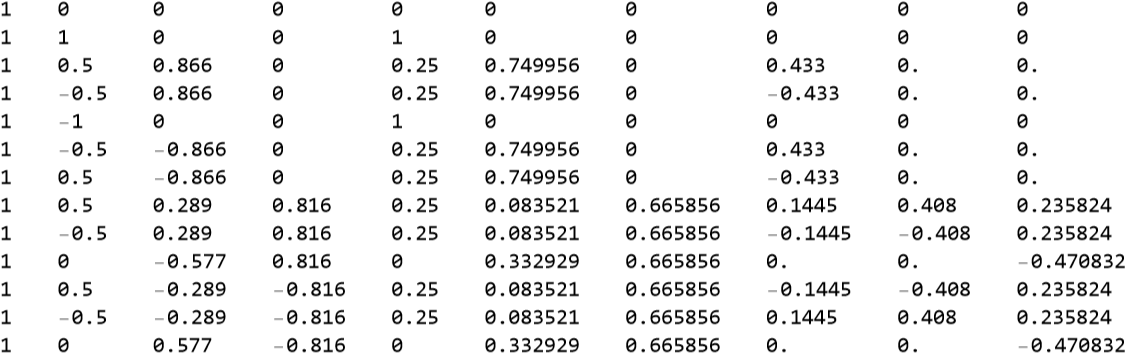
Determination of the quadratic model by multilinear regression of the mean particle size: = 1594 - 97.5 x + 117.6 x+ 16.7 x- 20.0 - 379.0 - 70.8 - 223.4 + 120.1 + 83.0 Results are in agreement with the model obtained by Lewis G. A., D. Mathieu and R. Phan-Than-Luu in Pharmaceutical Experimental Design, Drugs and the Pharmaceutical Sciences, Vol 92, 1999, Marcel Dekker, New York.
y
1
2
3
2
(x)
1
2
(x)
2
2
(x)
3
x
1
x
2
x
1
x
3
x
2
x
3
In[]:=
a=Inverse[Transpose[M].M].Transpose[M].y
Out[]=
{1594.,-97.5,117.639,16.7003,-20.,-379.022,-70.87,-223.441,120.189,83.0939}
Contour plots of the obtained mean size versus impeller speed (x1) and pelletization time (x3) for x2 (binding solution) =±0.5 and 0. We get the same figures as plotted in Figure 5.14 page 229 of the book by Lewis G. A., D. Mathieu and R. Phan-Than-Luu in Pharmaceutical Experimental Design, Drugs and the Pharmaceutical Sciences, Vol 92, 1999, Marcel Dekker, New York.
In[]:=
Clear[X2]
In[]:=
yp=1594-97.5X1-20.+117.6X2-223.4X1X2-379.+16.7X3+120.1X1X3+83.X2X3-70.8
2
X1
2
X2
2
X3
Out[]=
1594-97.5X1-20.+117.6X2-223.4X1X2-379.+16.7X3+120.1X1X3+83.X2X3-70.8
2
X1
2
X2
2
X3
In[]:=
X2=0.5;
In[]:=
p=ContourPlot[yp,{X1,-1,1},{X3,-1,1},Contours->15,Axes->False,PlotPoints->30,PlotRangePadding->0,Frame->False,ColorFunction->"DarkRainbow"];
In[]:=
p3=Plot3D[1594-97.5X1-20.+117.6X2-223.4X1X2-379.+16.7X3+120.1X1X3+83.X2X3-70.8,{X1,-1,1},{X3,-1,1},ColorFunction->"DarkRainbow"];
2
X1
2
X2
2
X3
In[]:=
level=1000;gr=Graphics3D[{Texture[p],EdgeForm[],Polygon[{{-1,-1,level},{1,-1,level},{1,1,level},{-1,1,level}},VertexTextureCoordinates->{{0,0},{1,0},{1,1},{0,1}}]},Lighting->"Neutral"];Show[p3,gr,PlotRange->All,BoxRatios->{1,1,.9},FaceGrids->{Back,Left}]
Out[]=
