Improved Supply and Demand Curves
Improved Supply and Demand Curves
The ordinary supply and demand graphs that I was taught in school involve two linear forces and their intersection.
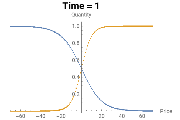
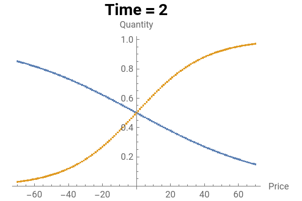
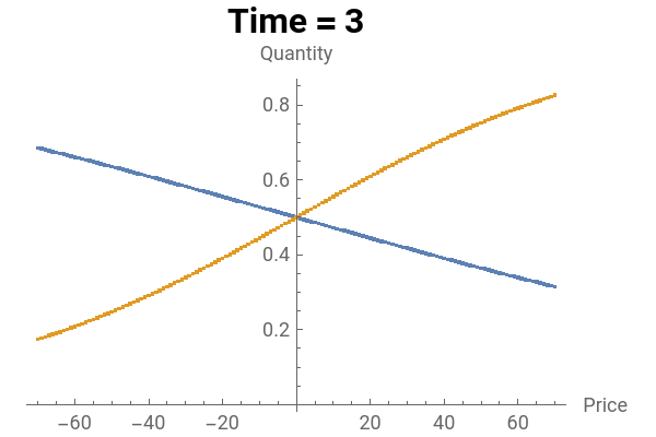
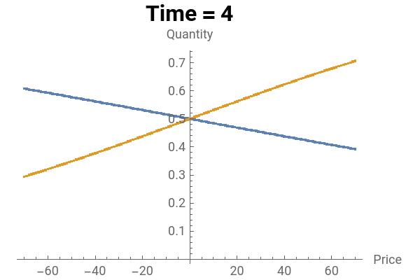
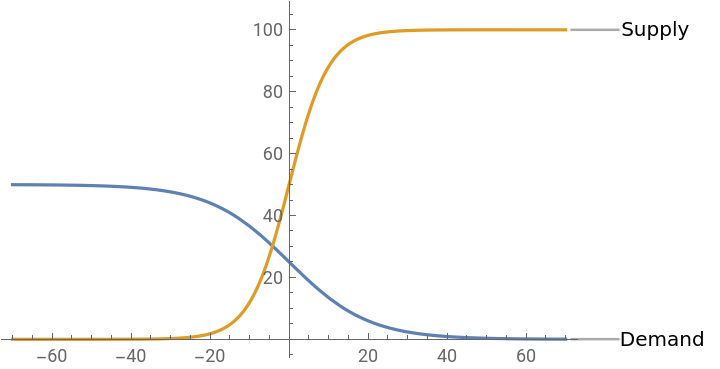
This more detailed supply and demand graph incorporates the concept of saturation, both for supply and demand.
In this model, supply & demand have limits and non-linear rates of change.
This more detailed supply and demand graph incorporates the concept of saturation, both for supply and demand.
In this model, supply & demand have limits and non-linear rates of change.
In[]:=
(*Definefunctionsfordemandandsupply*)demand[maxDemand_,rateChangeDemand_,price_]:=maxDemand/(1+Exp[-rateChangeDemand*price]);supply[maxSupply_,rateChangeSupply_,price_]:=maxSupply/(1+Exp[-rateChangeSupply*price]);(*Setparametervalues(adjusttheseasneeded)*)maxDemand=50;rateChangeDemand=-0.1;maxSupply=100;rateChangeSupply=.2;(*Definepricerangeforthegraph*)priceRange={-70,70};(*Generatedemandandsupplydatapoints*)demandPoints=Table[{price,demand[maxDemand,rateChangeDemand,price]},{price,priceRange[[1]],priceRange[[2]]}];supplyPoints=Table[{price,supply[maxSupply,rateChangeSupply,price]},{price,priceRange[[1]],priceRange[[2]]}];(*Createtheplot*)plot=Plot[{demand[maxDemand,rateChangeDemand,price],supply[maxSupply,rateChangeSupply,price]},{price,priceRange[[1]],priceRange[[2]]},PlotLabels->{"Demand","Supply"}];Show[plot]
Out[]=
In[]:=
Update
Out[]=
Update
In[]:=
(*Definefunctionsfordemandandsupply*)demand[changeDemand_,price_,time_]:=1/(1+Exp[-changeDemand/time^2*price]);supply[changeSupply_,price_,time_]:=1/(1+Exp[-changeSupply/time^2*price]);(*=======VariableDefinitions=======*)(*Rateofchangeindemand/supplywithrespecttopriceandtime*)changeDemand=-0.1;changeSupply=0.2;(*Definepricerangeandtimerangeforthegraph*)priceRange={-70,70};timeRange={1,10};(*Generatedemandandsupplydatapoints*)demandPoints=Flatten[Table[{price,time,demand[changeDemand,price,time]},{price,priceRange[[1]],priceRange[[2]]},{time,timeRange[[1]],timeRange[[2]]}],1];supplyPoints=Flatten[Table[{price,time,supply[changeSupply,price,time]},{price,priceRange[[1]],priceRange[[2]]},{time,timeRange[[1]],timeRange[[2]]}],1];(*Visualizethethree-dimensionalsupplyanddemandcurves*)ListPlot3D[{demandPoints,supplyPoints},PlotLegends->{"Demand","Supply"},AxesLabel->{"Price","Time","Quantity"}]
Out[]=


In[]:=
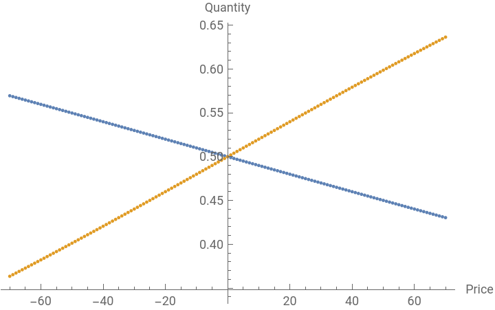
specificTime=5;(*Choosethedesiredtimevalue*)demandPointsAtTime=Table[{price,demand[changeDemand,price,specificTime]},{price,priceRange[[1]],priceRange[[2]]}];supplyPointsAtTime=Table[{price,supply[changeSupply,price,specificTime]},{price,priceRange[[1]],priceRange[[2]]}];ListPlot[{demandPointsAtTime,supplyPointsAtTime},PlotLegends->{"Demand","Supply"},AxesLabel->{"Price","Quantity"}]
Out[]=


In[]:=
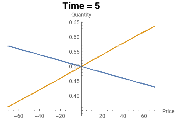
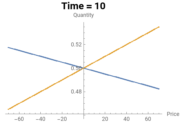
timePoints={1,2,3,4,5,10};snapshots=Table[ListPlot[{Table[{price,demand[changeDemand,price,time]},{price,priceRange[[1]],priceRange[[2]]}],Table[{price,supply[changeSupply,price,time]},{price,priceRange[[1]],priceRange[[2]]}]},PlotLegends->{"Demand","Supply"},AxesLabel->{"Price","Quantity"},ImageSize->{300,200},PlotLabel->Style["Time = "<>ToString[time],Bold,Black,16]],{time,timePoints}];gridLayout=Partition[snapshots,UpTo[3]];Grid[gridLayout,Frame->All,Spacings->1]
Out[]=