EnvelopeFamilySurfaces::usage="Find the envelope, the characteristics and the recoil edge of the surface family:x - C + (y - R + - ]x - C + (y + R + - ] = 0, ( + ≠ 0).References: Fedenko, A.S. Problemas de Geometría Diferencial. Editorial Mir: Moscú, p.85, 1981; Personal.";
2
)
2
)
2
z
2
R
2
)
2
)
2
z
2
R
2
y
2
z
Development:
In[]:=
Solve[(++-)(++-)==0,((++-)(++-))==0,{x,y}]
2
(x-c)
2
(y-R)
2
z
2
R
2
(x-c)
2
(y+R)
2
z
2
R
∂
c
2
(x-c)
2
(y-R)
2
z
2
R
2
(x-c)
2
(y+R)
2
z
2
R
Out[]=
xc,y-R--,xc,yR--,xc,y-R+-,xc,yR+-,{xc-z,y0},{xc+z,y0}
2
R
2
z
2
R
2
z
2
R
2
z
2
R
2
z
Envelope:
c,-R--,z;c,R--,z;c,-R+-,z;c,R+-,z;
2
R
2
z
2
R
2
z
2
R
2
z
2
R
2
z
Characteristic (for the element R = , c = 3):
2
3,-2-
4-
,z;3,2-2
z
4-
,z;3,-2+2
z
4-
,z;3,2+2
z
4-
,z;2
z
In[]:=
Reduce[4->=0,z]
2
z
Out[]=
-2≤z≤2
Recoil edge:
In[]:=
Solve(++-)(++-)==0,((++-)(++-))==0,((++-)(++-))==0,{x,y,z}
2
(x-c)
2
(y-R)
2
z
2
R
2
(x-c)
2
(y+R)
2
z
2
R
∂
c
2
(x-c)
2
(y-R)
2
z
2
R
2
(x-c)
2
(y+R)
2
z
2
R
∂
c,c
2
(x-c)
2
(y-R)
2
z
2
R
2
(x-c)
2
(y+R)
2
z
2
R
{{xc,y0,z0}};
But the text of the problem indicates +≠ 0, therefore we will not consider this point.
2
y
2
z
Graph:
In[]:=
ManipulateClearAll;ShowParametricPlot3D[{2Sin[u]Cos[v]+3,2Sin[u]Sin[v]+2,2Cos[u]},{u,0,π},{v,0,2πt1},PlotStyle->{Opacity[0.6],Red},MeshFalse,PerformanceGoal"Quality"],ParametricPlot3D[{2Sin[u]Cos[v]+3,2Sin[u]Sin[v]-2,2Cos[u]},{u,0,π},{v,0,2πt1},PlotStyle->{Opacity[0.6],Red},MeshFalse,PerformanceGoal"Quality"],ParametricPlot3Dc,-2-
4-
,z,{c,-2,6t1},{z,-2,2},PlotStyle->{Opacity[0.2],Yellow},MeshFalse,PerformanceGoal"Quality",ParametricPlot3Dc,2-2
z
4-
,z,{c,-2,6t1},{z,-2,2},PlotStyle->{Opacity[0.2],Yellow},MeshFalse,PerformanceGoal"Quality",ParametricPlot3Dc,-2+2
z
4-
,z,{c,-2,6t1},{z,-2,2},PlotStyle->{Opacity[0.2],Yellow},MeshFalse,PerformanceGoal"Quality",ParametricPlot3Dc,2+2
z
4-
,z,{c,-2,6t1},{z,-2,2},PlotStyle->{Opacity[0.2],Yellow},MeshFalse,PerformanceGoal"Quality",ParametricPlot3D3,-2-2
z
4-
,z,{z,-2,2t1},PlotStyle{Thickness[0.01],Blue},ParametricPlot3D3,-2+2
z
4-
,z,{z,-2,2t1},PlotStyle{Thickness[0.01],Blue},ParametricPlot3D3,2-2
z
4-
,z,{z,-2,2t1},PlotStyle{Thickness[0.01],Blue},ParametricPlot3D3,2+2
z
4-
,z,{z,-2,2t1},PlotStyle{Thickness[0.01],Blue},Graphics3D[{Black,Ball[{3,2,0},0.15]}],Graphics3D[{Black,Ball[{3,-2,0},0.15]}],AxesLabel->(Style[#,15,Blue]&/@{"X","Y","Z"}),AxesOrigin{0,0,0},AxesTrue,BoxedFalse,BoxRatiosAutomatic,PlotRangeAll,ViewPoint{-3,-2,1},ImageSize500,Style["Family of surfaces and envelope:",Bold,Large],{{t1,0.01,"Value (t1)"},0.01,1,0.01},ControlPlacementTop2
z
Out[]=


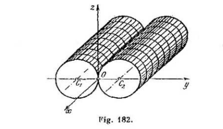
In the graph above you can see 2 elements of the family (spheres in red), the centers are the points in black, the characteristics in blue, the envelope are the cylinders in yellow. It has no recoil edge due to the conditions of the book.