ABSTRACT (original article): The shape of a microchannel is usually affected by a significant uncertainty due to the small size of the cross-section, comparable with the typical wall-roughness length scale. Such an uncertainty is present at any scale, but it is definitely amplified and, hence, significantly important when the hydraulic diameter becomes smaller than some tenth micrometers. The focus of this paper is on the numerical analysis of the sensitivity to shape random modification, within a prefixed maximum extent, of the main flow and heat transfer characteristics of fully-developed forced convection. The numerical solutions are carried out by employing a finite-element solver repeated over a statistical sample of randomly generated perimetral profiles that simulate the wall roughness. The study includes the evaluation of the Fanning friction factor and of the Nusselt number for the T, H1 and H2 thermal boundary condition. CITATION (original article): A. Barletta, M. Celli, L. A. Sphaier, P. V. Brandao, S. Lazzari, E. Ghedini (2024), Shape uncertainty analysis of laminar forced convection in a round microchannel with viscous dissipation, arXiv:2406.11348. https://doi.org/10.48550/arXiv.2406.11348
Dependent and independent variables
Dependent and independent variables
We start defining dependent and independent variable in a suitable fashion such that the writing of the governing equations results more readable
In[]:=
xx={x,y,z};vel={u1[x,y,z,t],u2[x,y,z,t],u3[x,y,z,t]};PP=p[x,y,z,t];TT=T[x,y,z,t];
Governing equations for a generic system
Governing equations for a generic system
Here we define the local balance equations: for future manipulation we define just the left handside of the homogeneous equations. We start from the Navier-Stokes equations for an incompressible and Newtonian fluid.
Local Mass Balance Equation: Continuity equation
In[]:=
em=Div[vel,xx];
Local Momentum Balance Equation: Incompressible Navier-Stokes equations
In[]:=
ev=ρ(D[vel,t]+vel.Transpose[Grad[vel,xx]])+Grad[PP,xx]-μLaplacian[vel,xx];
Local Energy Balance Equation: Conduction/Convection equation with viscous dissipation
In[]:=
ee=ρc(D[TT,t]+vel.Transpose[Grad[TT,xx]])-kLaplacian[TT,xx]-(D[vel[[i]],xx[[j]]]+D[vel[[j]],xx[[i]]])(D[vel[[i]],xx[[j]]]+D[vel[[j]],xx[[i]]]);
μ
2
3
∑
i=1
3
∑
j=1
Fully developed stationary flow: simplified equations
Fully developed stationary flow: simplified equations
Let (x, y) be the Cartesian coordinates on the cross-sectional plane and be the streamwise coordinate. The flow is assumed to be laminar, stationary, incompressible and fully-developed, so that the only nonzero component of the velocity field is that in the direction, which is denoted with . Due to the local mass balance equation, i.e. the zero-divergence condition on the velocity, is independent of , and hence . Furthermore, the local difference between the pressure and the hydrostatic pressure depends (linearly) only on . The thermal boundary conditions envisaged in this study are either , or according to the classification defined by Shah and London (Laminar Flow Forced Convection in Ducts, 1978). We recall that condition means a peripherally (along the perimeter of the cross section) and longitudinally (along ) uniform wall temperature, means a peripherally uniform wall temperature and a longitudinally uniform wall heat flux, while means a peripherally and longitudinally uniform wall heat flux. It is also well-known that conditions and coincide when the perimeter shape is exactly a circle (Shah and London, Laminar Flow Forced Convection in Ducts, 1978). Furthermore, the boundary conditions , or imply that the derivative is a constant, hereafter denoted as . More detailed information can be found in the ArXiv document https://arxiv.org/abs/2406.11348
z
z
u
u
z
u=u(x,y)
z
T
H
1
H
2
T
z
H
1
H
2
H
1
H
2
T
H
1
H
2
∂T/∂z
a
In[]:=
rulefd=List[u1Function[{x,y,z,t},0],u2Function[{x,y,z,t},0],u3Function[{x,y,z,t},u[x,y]],pFunction[{x,y,z,t},Pzz],TFunction[{x,y,z,t},az+T[x,y]]];em1=em/.rulefdev1=ev/.rulefdee1=ee/.rulefd
Out[]=
0
Out[]=
0,0,Pz-μ[x,y]+[x,y]
(0,2)
u
(2,0)
u
Out[]=
acρu[x,y]-μ2[x,y]+2[x,y]-k[x,y]+[x,y]
1
2
2
(0,1)
u
2
(1,0)
u
(0,2)
T
(2,0)
T
Dimensionless governing equations
Dimensionless governing equations
Here we define the transformations to obtain the dimensionless form of the equations.
(,)===kwith=-
x
y
(x,y)
r
0
u
u
u
0
T
T-
T
w
q
w
r
0
u
0
2
2
r
0
μ
p
z
The overlined quantities are dimensionless. In the code, we cut the overlines to simplify the treatment and we defined the dimensional quantities such that we can apply the following rules to manipulate the equations.
In[]:=
ruleadim1=uFunction[{x,y},u0u[x,y]],TFunction{x,y},T[x,y];ruleadim2=[x,y][x,y],[x,y][x,y],[x,y][x,y],[x,y][x,y],[x,y][x,y],[x,y][x,y];ruleu0=u0->-;
r0qw
k
(1,0)
u
(1,0)
u
r0
(0,1)
u
(0,1)
u
r0
(2,0)
u
(2,0)
u
2
r0
(0,2)
u
(0,2)
u
2
r0
(2,0)
T
(2,0)
T
2
r0
(0,2)
T
(0,2)
T
2
r0
2Pz
2
r0
μ
Applying the transformations and manipulating the left hand side of the equations
In[]:=
eud1=Simplify/.ruleu0ee2=ExpandFullSimplify
ev1[[3]]/.ruleadim1/.ruleadim2
2Pz
ee1/.ruleadim1/.ruleadim2
qw
r0
Out[]=
1
2
(0,2)
u
(2,0)
u
Out[]=
acr0u0ρu[x,y]
qw
2
u0
2
(0,1)
u
qwr0
(0,2)
T
2
u0
2
(1,0)
u
qwr0
(2,0)
T
Manipulation of the group parameters and definition of the Brinkman number Br and Poiseuille number σ
Br==a
μ
2
u
m
2
r
0
q
w
a
ρc
r
0
u
w
q
w
He we define the rule which allows us to employ the definitions just given
In[]:=
rule=u0->umσ,μ->2Br,->a;
2
um
qwr0
acr0umρ
qw
Applying the transformations and obtaining the ultimate version of dimensionless energi balance equations
In[]:=
euT1=-Expand[ee2//.rule]
Single solution: Nusselt values for T, H1 and H2 boundary conditions and random geometries
Single solution: Nusselt values for , and boundary conditions and random geometries
T
H
1
H
2
Loading of the Finite Element Method package
In[]:=
Needs["NDSolve`FEM`"]
Definition of the radius uncertainty (γγ) and of the number of points defining the geometry (nn)
rule0=γ->5,points->;
-2
10
2
10
Definition random coordinates of the points
nn=2π/points/.rule0;pts=Table[δφ=RandomReal[{0,nn}];AA=RandomReal[{-γ,γ}/.rule0];{(1+AA)Cos[φ+δφ],(1+AA)Sin[φ+δφ]},{φ,nn,2π,nn}];
Definition of the geometry
geo=Graphics[Polygon[pts]];region=Region@BoundaryDiscretizeGraphics@geo;
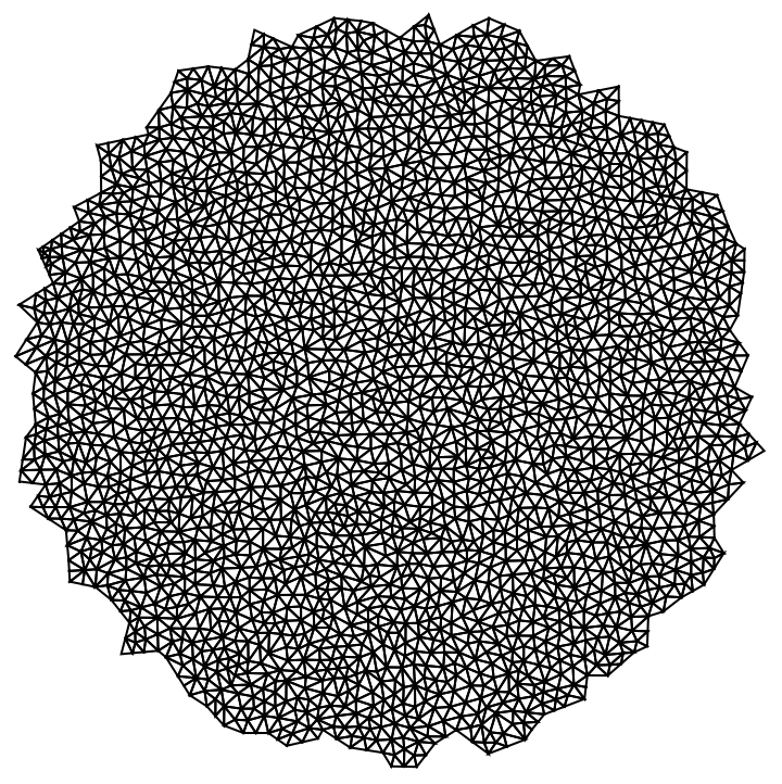
Definition of the mesh
reg=DiscretizeRegion[region];mesh=ToElementMeshreg,MaxCellMeasure->;mesh["Wireframe"]
-3
10
Out[]=
Solution of the velocity field over the geometry
Definition of the geometrical parameters (perimeter and surface), of the Poiseuille number (σ) and the Brinkman number for the T boundary condition (BrT)
Solution of the temperature field over the random geometry for the T boundary condition
Definition of Nusselt for the T boundary condition
Solution of the temperature field over the random geometry for the H1 boundary condition
Solution of the temperature field over the random geometry for the H2 boundary condition
Printing the results
Loop for a statistical sample of solutions
Loop for a statistical sample of solutions
Post-processing
Post-processing
Poiseuille number
Poiseuille number
CITE THIS NOTEBOOK
CITE THIS NOTEBOOK
Shape uncertainty analysis of laminar forced convection in a round microchannel with viscous dissipation
by Antonio Barletta, Michele Celli, Leandro Alcoforado Sphaier, Pedro Vayssiere Brandão, Stefano Lazzari & Emanuele Ghedini
Wolfram Community, STAFF PICKS, October 25, 2024
https://community.wolfram.com/groups/-/m/t/3308119
by Antonio Barletta, Michele Celli, Leandro Alcoforado Sphaier, Pedro Vayssiere Brandão, Stefano Lazzari & Emanuele Ghedini
Wolfram Community, STAFF PICKS, October 25, 2024
https://community.wolfram.com/groups/-/m/t/3308119