A single, fixed-radius deterministic cellular automaton cannot classify majority or plurality on a periodic ring using only local information, and this holds regardless of how many colors are involved. Splitting the task instead into a sort, a sequence of binary eliminations, and a vote across permutations of the colors allow us to construct a solution. Under this construction, 4 colors are classified correctly ~98% and 8 colors are classified correctly 99% of the time, and even a fixed sample of only 100 permutations, still gets 128 colors right several times more often than a random rule would.
Introduction
Introduction
The density classification task (DCT) is a benchmark for the computational capabilities of cellular automata operating under local rules. Given a binary array of length on a periodic ring, the task is to determine if the initial density of 1s is greater than 1/2 using only local interactions. If so, the entire array must converge to all 1s; otherwise, it must converge to all 0s. Let represent the density of a configuration . A cellular automaton solves the Density Classification Task (DCT) if it converges to the correct uniform state for any initial density
N
ρ(x)
1
N
∑
i
x
i
x∈
N
{0,1}
Φ
ρ(x)≠1/2
Land and Belew (1995) proved that no single cellular automaton rule with a fixed radius can solve the DCT with perfect accuracy for any ring size. Because of this, later research either accepted approximate solutions or used multiple rules.
The Gács-Kurdyumov-Levin (GKL) rule from 1978 is the most famous approximate solution. It achieves about 82% accuracy on random configurations. Later genetic algorithm searches (Mitchell, Crutchfield, and Das, 1996) found similar rules, but none significantly surpassed this 82% limit for a radius-3 (=3)rule.
r
If the restriction of using only a single rule is removed, perfect solutions become possible. Fukś (1997) demonstrated that applying two simple rules sequentially solves the binary DCT with 100% accuracy in time. First, Rule 184 groups the array into blocks. Then, Rule 232 (a simple majority rule) finds the majority on the grouped array.
O(N)
Extending the DCT to colors means the most frequent color (plurality) must be found instead of a simple binary majority. Chau, Siu, and Yan (1999) expanded the two-rule approach to any . Their method is 100% accurate, but the required rule radius grows with . Therefore, it cannot be implemented directly at a fixed scale.
k>2
k
N
This essay explores two main ideas. First, the binary case is revisited to identify the behavior of the GKL rule. For densities near , the GKL rule fails much more often on scattered (unsorted) configurations compared to sorted ones. This shows that sorting should be treated as its own distinct step.
ρ1/2
Second, this sorting concept is followed by a sequence of GKL-based eliminations, each round discarding half the remaining colors. This architecture is empirically verified for and .
k4
k8
The Binary Case Revisited
The Binary Case Revisited
Where GKL Breaks Down
Where GKL Breaks Down
The GKL rule achieves an accuracy rate of approximately 82% on random binary configurations of length N=149;which is consistent with the rate widely reported in the literature. However, a closer examination of its failures reveals a specific and exploitable structure. Two configurations containing the same number of 1s may differ in whether that majority is distributed across the ring or clustered in a single contiguous block. GKL performs significantly better in the latter case, yet the relationship between input arrangement and the outcome is not simply a matter of “ordered is better in every respect.” It reflects a speed-accuracy trade-off.
Figure 1: Chaotic vs. Sorted input, same majority count
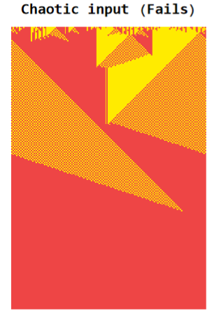
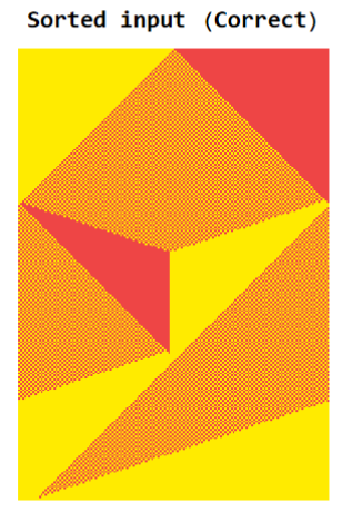
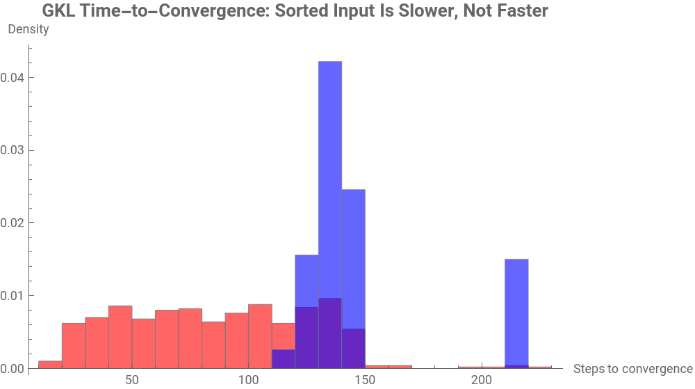
Measuring both convergence time and correctness across many random configurations makes the tradeoff explicit. Sorted inputs converge to the correct majority almost always (100% in this sample), against 84.6% for unsorted inputs at the same density — but sorted inputs take longer to converge: a mean of 145.9 steps versus 83.9 for unsorted inputs of the same size.
Figure 2: Time-to-convergence histogram, chaotic vs. sorted
Out[]=


The reason for the slowdown becomes clear once convergence time is examined as a function of the minority block’s size in a sorted configuration. For sorted inputs specifically, the ring reduces to exactly two contiguous blocks, and GKL’s dynamics must move the single boundary between them across the whole minority block before convergence. The larger that block, the longer this takes.
Figure 3: Minority block size vs. convergence time, sorted inputs
Out[]=
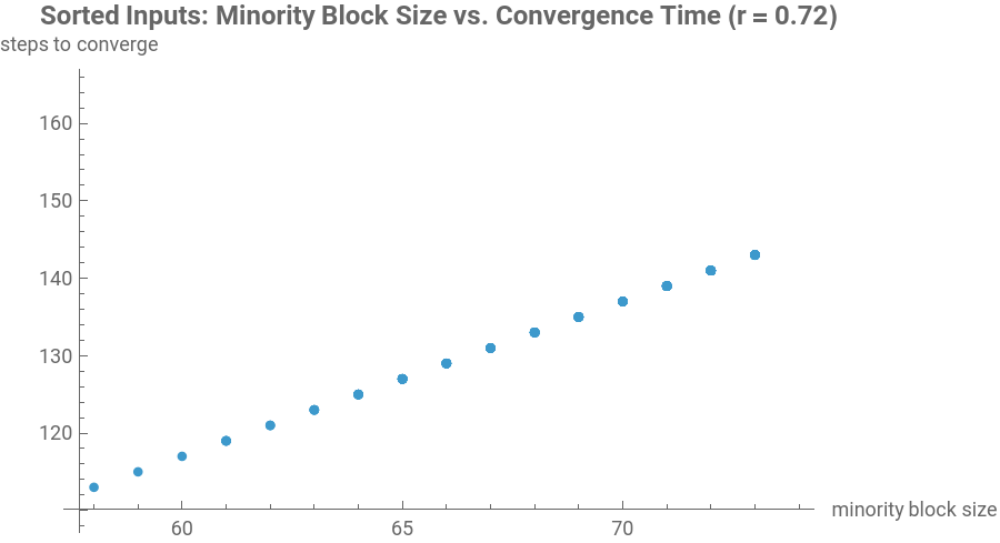
The correlation between minority block size and convergence time is strong (). Although sorting slows down the time to convergence, it increases accuracy significantly.
r≈0.72
Figure 4: Sorted vs. unsorted accuracy, same samples
Out[]=
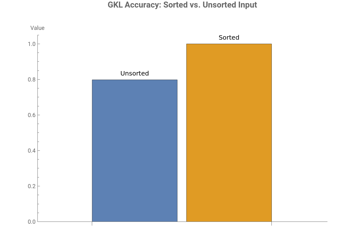


This situation allows for a reframing of the objective for the remainder of the essay.We are looking for an architecture that consciously accepts the time cost of the sorting process in exchange for the accuracy it yields and performs a separate, rapid consensus step once the input has already been organized into blocks.
A State-Graph View of GKL
A State-Graph View of GKL
The failures documented above raise a natural question. Is there some structural reason certain configurations are harder for GKL than others? Because the ring is periodic, this question has an answer at least for small . Circularity means many configurations are actually the same configuration. For instance; on a periodic ring, the array { } and the array { } describe the same physical arrangement of colors, the second is same with the first, read starting from a different cell. Since GKL treats these two arrays identically, its behavior can be revealed by analyzing necklaces, which are arrangements considered the same up to rotation, rather than raw arrays. Burnside’s Lemma gives the count of these necklaces.The number of distinct configurations on a ring of binary cells is φ(N/d)· where is Euler’s totient function.
N
1,1,0,0,1,0,1,0
0,0,1,0,1,0,1,1
N
1
N
∑
d|N
d
2
φ
Figure: raw configurations vs. distinct necklaces, N=8 to 16
N
2
Out[]=
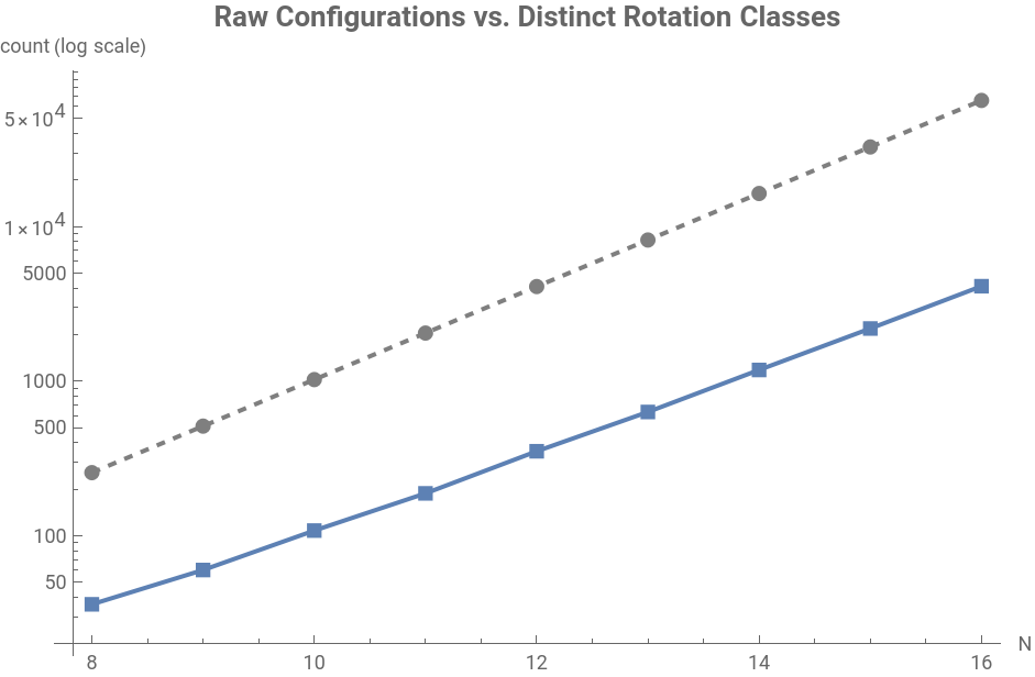


Because GKL maps each configuration to exactly one successor, the set of all necklaces and their GKL-successors forms a directed graph in which every node has exactly one outgoing edge. At, there are only 36 distinct necklaces and this can be easily visualized.
Because GKL maps each configuration to exactly one successor, the set of all necklaces and their GKL-successors forms a directed graph in which every node has exactly one outgoing edge. At
N8
Figure 5: the full necklace graph at N=8, colored by outcome.
Out[]=
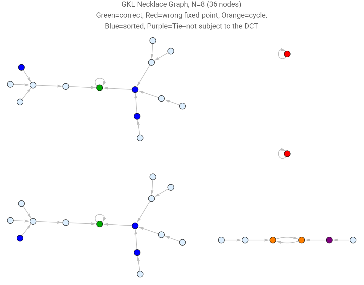
Figure 6: percent of states that never reach the correct answer, and the sorted-state “bottleneck” ratio, as N grows from 8 to 16
Figure 7: the full necklace graph at N=15
An Ensemble of Near-Optimal Rules
An Ensemble of Near-Optimal Rules
Figure 10: input where GKL fails but c6 succeeds
Figure 7: failure-overlap breakdown
Figure 11: GKL alone vs. speed-based ensemble, same test samples
Figure 12: GKL vs ensemble accuracy across N
The improvement is modest, and it does not point toward an exact solution. But it demonstrates that GKL’s errors are not a single monolithic failure mode. Different rules in GKL’s neighborhood fail on different inputs, in a way that a simple selection mechanism can partially exploit. This idea will be used in the later sections where adaptively searching is more expensive.
Radius Extension and Rule Degeneracy
Radius Extension and Rule Degeneracy
Figure 13: Degenerate rule, always converges to 2, regardless of input
This is a symptom of naive fitness design in the search. A fitness function that only rewards reaching a uniform state, without checking that the state matches the correct majority, is satisfied well by a rule that always converges to 0. The wider neighborhood at radius 4 makes the search harder, not more capable of true classification in this fitness function.
The k-ary Generalization Problem
The k-ary Generalization Problem
A Baseline k = 4 Rule and Its Bias
A Baseline k = 4 Rule and Its Bias
Figure 15: r4 per-color recall, quantifies the bias
What Goes Wrong in Fitness Function Design
What Goes Wrong in Fitness Function Design
Figure 16: best rule found under balancedFitnessK4, balanced across colors, but uniformly poor
Figure 17: best rule found across the full k=4 fitness-function search, the closest approach to balanced, correct performance, still short of random
Theoretical Limits: The Results of Chau–Siu–Yan
Theoretical Limits: The Results of Chau–Siu–Yan
The Impossibility Theorem
The Impossibility Theorem
An Empirical Verification of the Two-Rule Construction
An Empirical Verification of the Two-Rule Construction
Figure 18: Affinity phase then Propagation phase
Toward a Practical Construction
Toward a Practical Construction
Fukś (1997) showed that the binary density classification task, provably unsolvable by any single fixed-radius rule; however, it becomes solvable once the single-rule restriction is dropped. His construction runs two elementary rules in sequence. Rule 184 groups the ring without changing how many of each number there are. Rule 232 then completes the task. Given an already-sorted ring, a simple majority vote at each boundary is enough to push the whole ring to the correct color.
This result is the inspiration for the remainder of this essay.
This result is the inspiration for the remainder of this essay.
Figure 19: Fuks’ two-step binary construction
GKL is a more capable second-phase rule than plain majority. But it only knows how to choose between two options. Four colors need more than that. One way around this is to reuse GKL anyway, in stages. Split the four colors into two groups. Run GKL to pick a winning group. Then split that group in two, and run GKL again to pick a winner within it. This is what this essay call “tournament”: two rounds of binary elimination instead of one attempt at a four-way decision. Each round only needs GKL to answer which of two groups is more common instead of trying to rank four colors at once.
Figure 20: two-round bit-based tournament at k=4 & accuracy of it
The tournament reaches 57.4% accuracy, which is well above the 25% random accuracy. But it is still relatively low. This downside can be explained as follows: each round can only choose correctly between two groups if a cell can see which group its neighbors belong to. In a disordered ring, a given site’s seven neighbors can just as easily be split among all four colors. This prevents a high accuracy rate.
The Necessity of Sorting and Impossibility of Determinism
The Necessity of Sorting and Impossibility of Determinism
Motivation: Sorted vs. Unsorted Configurations
Motivation: Sorted vs. Unsorted Configurations
The tournament’s accuracy depends on how the colors are arranged, not just on how many of each are present. As we demonstrated for binary GKL, if the majority color is scattered across the ring, the first round often groups it with the wrong colors by accident. If the same colors are gathered into contiguous blocks, the majority forms one large block that the tournament mostly resolves correctly.
Figure 21: same true majority, unsorted vs. sorted, through the tournament. The plurality is orange in the initial case
Both rings start with the same count of each color. Only the arrangement differs, and the sorted one converges to the right answer.
Impossibility of Deterministic Ring Sorting
Impossibility of Deterministic Ring Sorting
A Stochastic Alternative
A Stochastic Alternative
Determinism is the specific point the proof above rules out. A rule that answers with a probability instead of a fixed value escapes it; since, it no longer has to give the same output every time it meets the same neighborhood. The two cases in the proof, the stable boundary and the disordered pair, can now come out differently.
In this model, each neighboring pair on the periodic ring is treated as a one-way valve with two flow settings. When encountering an out-of-order pair, the valve opens , swapping the cells with a high probability of 0.9 For an in-order pair, the valve remains mostly closed, however permits a minor swap probability of 0.05. This small probability plays a critical role. If this rate is set to zero, it behaves like deterministic case. While the ring never stops moving, it mostly remains in a dynamic equilibrium very close to a sorted state. This state is enough for enhancing the tournament.
Figure 22: sorting in action
Post-Sorting Tournament Performance
Post-Sorting Tournament Performance
Figure 23: tournament accuracy, unsorted vs. sorted input. Compare to Figure 18
Sorting first raises accuracy from 57.4% to ~70%. Most of the remaining failures share the same cause. In the first round, the majority color ends up paired with a minority color small enough that the pair still loses. The next section tries to find a solution to these wrong coalitions.
A Permutation Ensemble
A Permutation Ensemble
The failure type described in previous section arises because the tournament relies on a single alignment of the colors. Whether the majority color is eliminated in a given tournament round depends on which colors are grouped into the same coalition. The majority color can be trapped in a disadvantageous alliance, since this grouping is determined by a single mapping. Permuting this mapping before running the sort-and-tournament pipeline changes the coalitions in each round. Crucially, this permutation does not affect the physical density of the colors.
Figure 24: all six relabelings run on the same input, ensemble finds the majority with a high accuracy
Four of the six permutations converge to the correct color here (i.e. i = 1), two do not. Taking the majority color across all six gives the right answer despite those two individual failures.
Figure 25: ensemble accuracy, and how often it declines to answer
Once ties are separated, accuracy is 98% Ties are not wrong answers; they are the ensemble declining to pick, because the six permutations disagree.This happens when two colors are already close to equally common in the input, so a small shift in a permutation is enough to flip which one the tournament happens to favor. To check this, inputs are grouped by how close their top two colors are and look separately at the tie rate and the accuracy within each group.
Figure 26: tie rate and accuracy, plotted against how close the top two colors are
As the figure shows, ties mostly occur when the ratios of the two colors are very close to each other.
Figure 27: sort, then 3 tournament rounds
The Statistical Mechanism Behind the Improvement
The Statistical Mechanism Behind the Improvement
Figure 28: single-permutation accuracy vs. random baseline vs. full ensemble
Figure 29: accuracy vs. ensemble size
Each point in Figure 29 is the accuracy measured at one particular ensemble size, from a single permutation up to the full 5040. The dashed gray line marks the 12.5% random-guess baseline. A modest ensemble mostly figures out the problem, and most of the remaining gap closes before the full factorial ensemble is needed.
Limitations at Large k and a Monte Carlo Approximation
Limitations at Large k and a Monte Carlo Approximation
Figure 30: accuracy at a fixed Monte Carlo Ensemble (M=100)
Asymptotic Complexity of the Final Solution
Asymptotic Complexity of the Final Solution
Stochastic Sorting
Stochastic Sorting
Tournament GKL
Tournament GKL
Full Permutation Ensemble Execution
Full Permutation Ensemble Execution
Monte Carlo Ensemble Execution
Monte Carlo Ensemble Execution
Concluding Remarks
Concluding Remarks
Density classification looks simple on paper, but is a genuinely hard task once information is restricted to local neighbors. The adaptive searches repeatedly showed how fragile this is. Even a small flaw in the fitness function was enough to produce rules that ignored the input and collapsed onto a single, biased color. The radius required for an exact solution also grows astronomically with the number of colors. This makes it computationally very expensive. Also hand-engineering a rule is difficult in its own right, since cellular automaton behavior is hard to predict from its rule table alone. This is part of why a divide-and-conquer approach was chosen over a search for a single rule.
Acknowledgments
Acknowledgments
References
References
1. Chau, H. F., Siu, T. K., & Yan, K. K. (1999). One-dimensional n-state cellular automaton solution to the density classification problem. International Journal of Modern Physics C, 10(5), 883–889.
2. de Oliveira, P. P. B. (2014). On density determination with cellular automata: Results, constructions and directions. Journal of Cellular Automata, 9(5–6), 357–385.
3. Fukś, H. (1997). Solution of the density classification problem with two cellular automata rules. Physical Review E, 55(3), R2081–R2084. https://doi.org/10.1103/PhysRevE.55.R2081
4. Gács, P., Kurdyumov, G. L., & Levin, L. A. (1978). One-dimensional uniform arrays that wash out finite islands. Problemy Peredachi Informatsii, 14(3), 92–96.
5. Land, M., & Belew, R. K. (1995). No perfect two-state cellular automata for density classification exists. Physical Review Letters, 74(25), 5148–5150. https://doi.org/10.1103/PhysRevLett.74.5148
6. Wolfram, S. (2021, May 17). The problem of distributed consensus. Stephen Wolfram Writings. https://writings.stephenwolfram.com/2021/05/the-problem-of-distributed-consensus/
AI Disclosure
AI Disclosure
The following generative AI tools were used in this project: Claude Sonnet 4.6 and Claude Sonnet 5. They were used for debugging and cleaning up code, and editing the essay’s prose. All code and written content was reviewed, understood, and approved by the author.
CITE THIS NOTEBOOK
CITE THIS NOTEBOOK
Solving the k-ary Density Classification Task
by Ahmet Erhan AVCI
Wolfram Community, STAFF PICKS, July 16, 2026
https://community.wolfram.com/groups/-/m/t/3762406
by Ahmet Erhan AVCI
Wolfram Community, STAFF PICKS, July 16, 2026
https://community.wolfram.com/groups/-/m/t/3762406