I wanted to understand more how the (discrete) Elliptic Curve algorithm(s) works, and did some experiments. Here are some of them. The inspiration for this was reading “Cryptography - Theory and Practice” (1995) by Douglas R. Stinson. The algorithm is described in Section “5.2.2 Elliptic Curves” (page 183ff).
I have not explained all the steps and algorithms used below, and I might very well have misunderstood some (finer) aspects of this. Please see Stinson or some other Cryptography book for details about this. Also, the specific implementations used here don’t scale and will not be of much use in a real crypto system.
I have not explained all the steps and algorithms used below, and I might very well have misunderstood some (finer) aspects of this. Please see Stinson or some other Cryptography book for details about this. Also, the specific implementations used here don’t scale and will not be of much use in a real crypto system.
Elliptic CurvesAn elliptic curve is described as y^2 = x^3 + a x + b mod pwhere 4 a^3 + 27b^2 != 0 mod pThe example Stinson works with (page 183ff) is y^2 = x^3 + x + 6i.e. a = 1 and b = 6.
The basic tool used is Mathematica’s Solve[] function with the Modulus option.
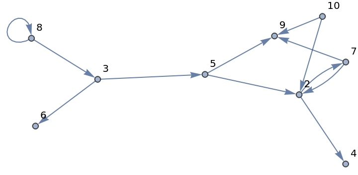
There are 12 solutions (12 points, {x1,y1}, {x2,y2},....) to this equation, shown as a table and as a graph: each “point” is a directed edge from one node to another (the x and y components). (As it happens this graph is connected but it don’t seems to be in the general case.)
There are 12 solutions (12 points, {x1,y1}, {x2,y2},....) to this equation, shown as a table and as a graph: each “point” is a directed edge from one node to another (the x and y components). (As it happens this graph is connected but it don’t seems to be in the general case.)
In[]:=
s=Solve[y^2==x^3+x+6,{x,y},Modulus11]Length@sTableForm[t={#[[1,2]],#[[2,2]]}&/@s]g=#[[1,2]]->#[[2,2]]&/@sGraph[g,VertexLabels"Name"]
Out[]=
{{x2,y4},{x2,y7},{x3,y5},{x3,y6},{x5,y2},{x5,y9},{x7,y2},{x7,y9},{x8,y3},{x8,y8},{x10,y2},{x10,y9}}
Out[]=
12
Out[]//TableForm=
2 | 4 |
2 | 7 |
3 | 5 |
3 | 6 |
5 | 2 |
5 | 9 |
7 | 2 |
7 | 9 |
8 | 3 |
8 | 8 |
10 | 2 |
10 | 9 |
Out[]=
{24,27,35,36,52,59,72,79,83,88,102,109}
Out[]=
The important concept for Elliptic Curves is a generator “a” (concept from group theory), which is a point which generates all other points when doing “powers” of a, i.e. a, a^2, a^3, ... .
The definition of this “addition” of two points - (x1,y1) + (x2,y2) - is a little complex, but the implementation below seems to work. It’s from page 184 in Stinson.
The division in the algorithm (Stinson page 184) is the multiplicative inverse (using Mathematica’s ModularInverse[n,mod]), and everything is done modulo Mod.
I’m not sure how to best represent the “Infinity” (“O”, identity), so it’s just an empty list which works quite well when using NestWhileList[] below.
The “infinity” occurs when
x2 == x1 and y2 == -y1 modulo mod
For a point P, the following holds
P + O = O + P = P
thus O is the identity element in this group.
Using this method we can generate all points until we get this “infinity” (identity) element.
In[]:=
add[{x1_,y1_},{x2_,y2_},a_,m_]:=Module[{x3,y3,λ},If[x1==x2&&y2==Mod[-y1,m],{},(*"Infinity"/"Identity"*)If[{x1,y1}=={x2,y2},λ=Mod[(3*x1^2+a)ModularInverse[2*y1,m],m],λ=Mod[(y2-y1)ModularInverse[x2-x1,m],m]];x3=Mod[λ^2-x1-x2,m];y3=Mod[λ*(x1-x3)-y1,m];{x3,y3}]]
Stinson shows (page 185f) how the generator (2,7) is evolving using the power operations. The first few powers for the elliptic curve equation above. The last addition - (2,4) + (2,7) - is the end of the sequence, i.e. it give “infinity” as result. This is because it now satisfies the test:
x1 == x2 && y2 = Mod[-y1,11]
i.e.
2 == 2 && 7 == Mod[-4,11]
x1 == x2 && y2 = Mod[-y1,11]
i.e.
2 == 2 && 7 == Mod[-4,11]
In[]:=
add[{2,7},{2,7},1,11]add[%,{2,7},1,11]add[%,{2,7},1,11]add[%,{2,7},1,11]Print["..."]add[{5,9},{2,7},1,11]add[{2,4},{2,7},1,11]
Out[]=
{5,2}
Out[]=
{8,3}
Out[]=
{10,2}
Out[]=
{3,6}
...
Out[]=
{2,4}
Out[]=
{}
The last point (2,4) is the "inverse" of the start point (2,7), with some modulus. inv[] is defined below and is (also) used for doing subtraction (the inverse of addition) of two points later on.
In[]:=
inv[{x_,y_},m_]:=Mod[{x,-y},m]
In[]:=
inv[{2,7},11]
Out[]=
{2,4}
Let’s use NestWhileList[] to see the full sequence (evolution).
Here one can note that the list plot don’t show the nice curves that the real valued version of elliptic curves shows, but we can see the mirror aspect in the plot (each y has two solutions).
Most[] is to used for getting rid of the “infinity” marker ({}) when plotting etc.
Remember: The generator a is (2,7).
In[]:=
add2[{x1_,x2_}]:=add[{x1,x2},{2,7},1,11](s=NestWhileList[add2,{2,7},#!={}&])//TableFormListLinePlot[Most[s]]
Out[]//TableForm=
2 | 7 |
5 | 2 |
8 | 3 |
10 | 2 |
3 | 6 |
7 | 9 |
7 | 2 |
3 | 5 |
10 | 9 |
8 | 8 |
5 | 9 |
2 | 4 |
Out[]=
Another - slightly larger - exampleLet’s try a slightly larger example (I’ve forgot the source for this equation, it’s not from Stinson): y^2 = x^3 + 9x + 17 mod 23 a = 9, b = 17 There are 31 solutions/points for this equation.
In[]:=
s=Solve[{y^2==x^3+9x+17},{y,x},Modulus->23];Length@st={#[[1,2]],#[[2,2]]}&/@st//TableFormg=#[[1,2]]->#[[2,2]]&/@sGraph[g,VertexLabels"Name"]
Out[]=
31
Out[]=
{{0,17},{2,1},{3,7},{3,19},{3,20},{5,3},{5,4},{5,16},{6,12},{7,5},{7,8},{7,10},{9,14},{10,13},{10,15},{10,18},{13,13},{13,15},{13,18},{14,14},{16,5},{16,8},{16,10},{17,12},{18,3},{18,4},{18,16},{20,7},{20,19},{20,20},{21,1}}
Out[]//TableForm=
0 | 17 |
2 | 1 |
3 | 7 |
3 | 19 |
3 | 20 |
5 | 3 |
5 | 4 |
5 | 16 |
6 | 12 |
7 | 5 |
7 | 8 |
7 | 10 |
9 | 14 |
10 | 13 |
10 | 15 |
10 | 18 |
13 | 13 |
13 | 15 |
13 | 18 |
14 | 14 |
16 | 5 |
16 | 8 |
16 | 10 |
17 | 12 |
18 | 3 |
18 | 4 |
18 | 16 |
20 | 7 |
20 | 19 |
20 | 20 |
21 | 1 |
Now we pick some of these points as a start point, say (20,19), and see what happens.
Ah, this is a little more like the real valued elliptic curves. :-)
Ah, this is a little more like the real valued elliptic curves. :-)
But we want the generator what generates (traverses) all the points. So let' s brute force it by trying all the points from the solution space as start points. (There are probably some much more efficient and nifty group theoretic methods to find this generator, but my basic group theory knowledge fails me here.)
The genSeq[] generates all the points when doing powers from the initial point {x1,y1}.
The genSeq[] generates all the points when doing powers from the initial point {x1,y1}.
To save space, only the longest sequences are shown here.
This shows that a=(2,1) is the generator we looked for and (2,22) is the last point (the inverse).
Here is a nicer table as well as a plot .
(It’s interesting that the sequence of x’s in the two generated tables are palindromes. This is probably not a coincidence, but I’m not sure how to interpret/prove this.)
A small crypto example
In page186f (example 5.8), Stinson describes how to use this to encrypt/decrypt a simple message.
The example uses with the first elliptic equation above: y^2 = x^3 + x + 6
Suppose that the generator α = (2,7) and Bob’s secret “exponent” is a=7, so
β = 7*α = 7(2,7) = (2,7)^7 = (7,2)
Note: Stinson use the notation
k(x,y)
for (x,y)^k i.e. the k’th power of a point.
The encryption operation is
enc(x,k) = (k(2,7), x+k(7,2))
and the decryption operation is
dec(y1,y2) = y2 - 7*y1
Suppose that Alice wishes to encrypt the message x = (10,9) (which is a point in E).
If she chooses the random value k=3, then she will compute:
y1 = 3(2,7) = (8,3) i.e. (2,7)^3
y2 = (10,9) + 3(7,2) = (10,2)
Hence the ciphertext is y = ((8,3),(10,2))
Now, if Bob receives the ciphertext, he decrypt it as follows:
plaintext = (10,2) - 7(8,3) = (10,9)
For doing these calculations we need a function of “power” of a point p modulo m and with the equation coefficient a,
called pow[] here. It just loops k times and returns the found point after k-1 steps.
called pow[] here. It just loops k times and returns the found point after k-1 steps.
Thus (2,7)^7 mod 11 given this equation is (7,2).
Alice’s part: decrypt the message (10,9)
Bob’s part: decrypt Alice’s message
x = decrypted = (10,2) - 7(8,3) = (10,9)
Here the subtraction -7(8,3) is the inverse of 7(8,3) using inv[] defined above.
x = decrypted = (10,2) - 7(8,3) = (10,9)
Here the subtraction -7(8,3) is the inverse of 7(8,3) using inv[] defined above.
Final words
After that Stinson (page 188ff) describes more complex algorithms to create a elliptic curve cryptosystem. But now I’ve understood enough of the basic principles of elliptic curves, so I end these experiments.
After that Stinson (page 188ff) describes more complex algorithms to create a elliptic curve cryptosystem. But now I’ve understood enough of the basic principles of elliptic curves, so I end these experiments.