ABSTRACT (original article): One of the latest predictions of Einstein’s theory is the existence of wormholes (WHs). In this work, we present exact solutions of the Einstein-Maxwell-dilaton equations representing traversable wormholes. These solutions satisfy the energy conditions and have a ring singularity satisfying the cosmic censorship of WHs, i.e., we show that, as in previous solutions, geodesics cannot touch the singularity. We delineate the optimal traversal regions for two classes of solutions. The solution referenced in 𝜆5 allows for secure passage in proximity to the poles and the equatorial plane. Conversely, the solution in 𝜆𝑁1 tends to favor trajectories near the poles and the equatorial plane; however, it affords greater flexibility. This study shows that solutions incorporating a dilatonic scalar field satisfy the null energy condition. We also find that the solution associated with the first class is physically feasible, while for the second class it presents the problem of not being asymptotically flat when considering a dilatonic-type scalar field. Finally, we give examples of realistic astrophysical objects that could fulfill these conditions. CITATION (original article): Leonel Bixano, Tonatiuh Matos (2025), Phys. Rev. D 111, 084056. https://doi.org/10.1103/PhysRevD.111.084056
Attached at the end of this post the notebooks of the following
◼
Verification that our solutions satisfy the Einstein–Maxwell–Dilaton field equations, together with the computation of all relevant geometric quantities associated with the solutions.
◼
Geodesic plots and analysis.
◼
Wormhole profile plots.
◼
Tidal force plots.
Comparative Numerical Visualization of the L5 and LN1 Solutions
Comparative Numerical Visualization of the L5 and LN1 Solutions
This section consolidates the numerical visualization procedures for the L5 and LN1 solutions. Each branch is evaluated independently with its original parameter values and branch-specific analytic expressions. For y = 0.25, 0.50, 0.75, and 0.90, the code constructs the auxiliary functions, solves the differential equation z^2= F-G subject to z(0) = 0, samples the corresponding ρ and z values, and generates both individual and superposed profiles. The two implementations are retained as separate evaluation groups because they intentionally reuse the same Mathematica symbols.
Evaluation note: run each solution group from top to bottom and complete its combined plot before evaluating the next group.
First Solution: L5 Branch
λ6+λ5=λ0y2L2x+2y+τ0x/L2x+2y;
λ
6
λ
5
λ0++τ0+;
y
2
L
2
x
2
y
x/L
2
x
2
y
This block evaluates the L5 branch. In the adopted parameterization in the article, while the numerical domain is x in [-25, 25] with step size x = 0.1.
Parameter Values
Parameter Values
The initialization cell assigns the characteristic scale L, the coupling K0, the branch parameters, the normalization f0, and the numerical integration interval. These quantities are subsequently used by the iterative solver and by all plotting cells in this block.
In[]:=
L=10;K0=1/12;τ0=1/10^2;λ0=0;f0=1;x0=-25;x1=25;DeltaX=0.1;
Iterative Numerical Procedure
Iterative Numerical Procedure
For each prescribed value of y, the Do loop evaluates the branch-specific expressions for ω, k, and ρ and constructs the derived quantities F and G. NDSolve then integrates z^2 = F -G with the initial condition z(0) = 0. The resulting numerical solution is sampled over the selected x interval, and Switch stores each dataset in a dedicated variable associated with y = 0.25, 0.50, 0.75, or 0.90.
Doy0=i;(*Definicióndelasformulas*)ω=L;k=-*()*((1-)*(((1-)+2(+))-8(+1)))+*(1-)*(8(+1)-(1-))+(8xy(1-)(+1)(-)*(τ0*λ0));ρ=Sqrt[(+1)(1-)-];F=L^2*++1*Exp[2k/.{y->y0}];G=;(*Resolucióndelaecuacióndiferencial*)sol=NDSolve[{(z'[x])^2==F-G,z[0]==0},z,{x,x0,x1,DeltaX}][[1]];(*Construccióndelalista*)listaRhoZ=Table[{ρ/.{x->xval},z[xval]/.sol},{xval,x0,x1,DeltaX}];(*Asignacióndelalistaavariablesdiferentessegúnelvalordey0*)Switch[y0,0.25,listaRhoZ25=listaRhoZ,0.5,listaRhoZ5=listaRhoZ,0.75,listaRhoZ75=listaRhoZ,0.9,listaRhoZ9=listaRhoZ],{i,{0.25,0.5,0.75,0.9}}(*FindelDo*)
(x-x)λ0-(1+)yτ0
2
y
2
x
(+)
2
x
2
y
K0
4
2
τ0
2
y
2
(+)
2
x
2
y
2
y
2
x
2
y
2
x
2
y
2
x
4
(+)
2
x
2
y
2
(λ0)
1
4
(+)
2
x
2
y
2
y
2
x
2
y
2
x
2
y
2
(+)
2
x
2
y
2
y
2
x
2
x
2
y
4
(+)
2
x
2
y
2
L
2
x
2
y0
2
(ω/.{y->y0})
2
x
2
y0
2
x
2
D(+1)(1-)-,x
2
L
2
x
2
y0
2
(ω/.{y->y0})
Individual Profiles
Individual Profiles
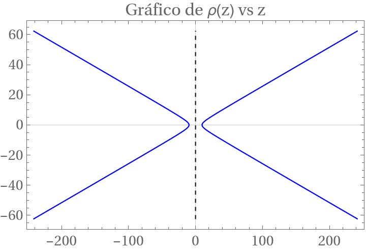
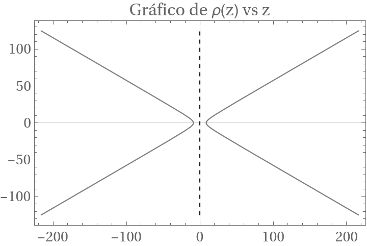
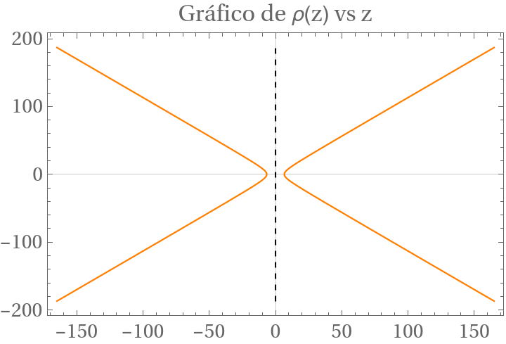
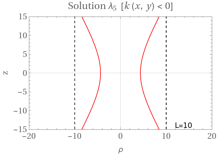
Each subsection constructs a ListLinePlot for one value of y. The original dataset and its sign-reversed counterpart are plotted together to display the two symmetric branches. The legends, reference lines, plot ranges, scientific theme, and original graphical formatting are retained.
y
0
Grafica25=ListLinePlot{-listaRhoZ25,listaRhoZ25},
Out[]=

y
0
Grafica5=ListLinePlot{-listaRhoZ5,listaRhoZ5},
Out[]=

y
0
Grafica75=ListLinePlot{-listaRhoZ75,listaRhoZ75},
Out[]=

y
0
Grafica9=ListLinePlot{-listaRhoZ9,listaRhoZ9},
Out[]=

Combined Visualization and Export
Combined Visualization and Export
Show superposes the four previously generated L5 graphics in a single visualization. The assembled figure is exported at an image resolution of 800 using the relative filename Lambda5-VariasYs.png.
CombinacionG=Show[Grafica9,Grafica75,Grafica5,Grafica25]Export["Lambda5-VariasYs.png",CombinacionG,ImageResolution->800];
Second Solution: LN1 Branch
This block evaluates the LN1 branch. In the adopted parameterization, x0 = -10 and x1= 10, while the numerical domain is x in [-10, 10] with step size x = 0.05. The definitions of ω(x,y), k(x,y), ρ(x,y), F, and G are preserved exactly as supplied.
Parameter Values
Parameter Values
The initialization cell assigns the characteristic scale L, the coupling K0, the branch parameters, the normalization f0, and the numerical integration interval. These quantities are subsequently used by the iterative solver and by all plotting cells in this block.
Iterative Numerical Procedure
Iterative Numerical Procedure
For each prescribed value of y, the Do loop evaluates the branch-specific expressions for ω, k, and ρ and constructs the derived quantities F and G. NDSolve then integrates z^2= F-G with the initial condition z(0) = 0. The resulting numerical solution is sampled over the selected x interval, and Switch stores each dataset in a dedicated variable associated with y= 0.25, 0.50, 0.75, or 0.90.
Individual Profiles
Individual Profiles
Each subsection constructs a ListLinePlot for one value of y. The original dataset and its sign-reversed counterpart are plotted together to display the two symmetric branches. The legends, reference lines, plot ranges, scientific theme, and original graphical formatting are retained.
Combined Visualization and Export
Combined Visualization and Export
Show superposes the four previously generated LN1 graphics in a single visualization. The assembled figure is exported at an image resolution of 800 using the relative filename LambdaN1-VariasYs.png.
Null Energy Condition Analysis
Null Energy Condition Analysis
This section evaluates and visualizes the quantity denoted rho - P in the code for the L5 and LN1 solutions. The analysis is numerical and graphical: it studies the sign and magnitude of the expression over specified coordinate domains and parameter choices rather than providing a symbolic proof of an energy condition.
Interactive plots are used for parameter exploration, while fixed-parameter surfaces and contour maps are used for direct comparison.
L5 solution: preliminary NEC visualization
L5 solution: preliminary NEC visualization
This block explores the diagnostic quantity labeled rho - P for the L5 solution. The scale parameters are fixed to L = 1 and tau0 = 1. The first surface uses k0 = -1/4, the interactive surface and contour plots vary k0 from -1 to 1, and the remaining cells examine selected fixed values together with the y = 0 section.
LN1 solution: preliminary NEC visualization
LN1 solution: preliminary NEC visualization
This block provides the corresponding exploratory analysis for the LN1 solution with L = 1 and lambda0 = 1. The interactive surface and contour plots vary k0 from -1 to 1 in increments of 1/4. The color prescription separates negative values of the plotted expression from nonnegative values.
L5 solution: fixed-parameter NEC comparison
L5 solution: fixed-parameter NEC comparison
This section generates publication-oriented L5 figures for k0 = -1/2, -1/4, and 1/12. For each parameter value, a three-dimensional surface is paired with a contour map so that the magnitude and spatial sign structure can be compared directly.
Three-dimensional surfaces
Three-dimensional surfaces
Each Plot3D cell evaluates the L5 expression over the specified coordinate domain and stores the resulting graphic. Blue is assigned to negative values, while the nonnegative region is represented by the remaining color scale.
Contour maps and combined figure
Contour maps and combined figure
Each ContourPlot cell gives a two-dimensional sign map of the same L5 expression. The GraphicsGrid cell combines every surface with its corresponding contour map, and the final Export command saves the assembled figure in the current working directory.
LN1 solution: fixed-parameter NEC comparison
LN1 solution: fixed-parameter NEC comparison
This subsection repeats the fixed-parameter analysis for the LN1 solution at k0 = -1/2, -1/4, and 1/12. The paired surface and contour representations allow the two-dimensional sign distribution to be compared with the full three-dimensional profile.
Three-dimensional surfaces
Three-dimensional surfaces
Each Plot3D cell evaluates the LN1 expression over the selected coordinate domain and stores the graphic for later assembly. The color rule highlights negative values in blue and displays nonnegative values with the remaining scale.
Contour maps and combined figure
Contour maps and combined figure
Each ContourPlot cell displays the spatial sign structure of the LN1 expression. The GraphicsGrid cell arranges the three surface-contour pairs, and the final Export command writes the collection to the current working directory.
CITE THIS NOTEBOOK
CITE THIS NOTEBOOK
Einstein-Maxwell-dilaton wormholes that meet the energy conditions
by Leonel Bixano & Tonatiuh Matos
Wolfram Community, STAFF PICKS, July 6, 2026
https://community.wolfram.com/groups/-/m/t/3745366
by Leonel Bixano & Tonatiuh Matos
Wolfram Community, STAFF PICKS, July 6, 2026
https://community.wolfram.com/groups/-/m/t/3745366