According to WMO: “The World Meteorological Organization (WMO) has confirmed that 2024 is the warmest year on record, based on six international datasets. The past ten years have all been in the Top Ten, in an extraordinary streak of record-breaking temperatures.”
According to NASA: “Earth’s average surface temperature in 2024 was the warmest on record, according to an analysis led by NASA scientists. Global temperatures in 2024 were 2.30 degrees Fahrenheit (1.28 degrees Celsius) above the agency’s 20th-century baseline (1951-1980), which tops the record set in 2023. The new record comes after 15 consecutive months (June 2023 through August 2024) of monthly temperature records — an unprecedented heat streak.”
Ten years ago Marco Thiel created spiral and annual window animations for global temperature rise. Since 2024 as the hottest year on record, I remade one with a bit different dataset that spans back to 1750.
Berkeley Earth Dataset: High-Resolution Global Land Only (Experimental; 1750 – Recent)
Berkeley Earth Dataset: High-Resolution Global Land Only (Experimental; 1750 – Recent)
Note from Berkeley Earth: “Berkeley Earth provides high-resolution land and ocean time series data and gridded temperature data. Our peer-reviewed methodology incorporates more temperature observations than other available products, and often has better coverage. Global datasets begin in 1850, with some land-only areas reported back to 1750. The newest generation of our products are augmented by machine learning techniques to improve the spatial resolution. This allows Berkeley Earth to provide the most comprehensive, high-resolution instrumental temperature data product available.”
Dataset copy at NOAA:
Note from berkeleyearth.org: “This file is based on the new high-resolution Berkeley Earth global temperature data set. It expands upon the previous Berkeley Earth temperature data set by including predictive structures based on historical weather patterns and increasing the underlying resolution to 0.25° x 0.25° latitude-longitude. Files based on this new data set are being provided as part of an early preview to aid in the identification of any remaining bugs or errors. While, we believe the current data set to be accurate and useful, it is still in development and substantial revisions remain possible if significant issues are identified. This file contains a detailed summary of the land-surface average results produced by the Berkeley Averaging method. Temperatures are in Celsius and reported as anomalies relative to the Jan 1951-Dec 1980 average. Uncertainties represent the 95 confidence interval for statistical and spatial undersampling effects.”
In[]:=
url="https://storage.googleapis.com/berkeley-earth-temperature-hr/global/Land_TAVG_monthly.txt";
Let's begin by importing the Berkeley Earth dataset, which contains high-resolution global land temperature data from 1750 to the present. This dataset provides temperature anomalies relative to the 1951–1980 average and is valuable for analyzing historical temperature changes.
In[]:=
rawDATA=Import[url,"Table"]
Out[]=
Next, we construct a object from the imported data. By doing this, we can efficiently handle and analyze temporal data, allowing us to explore temperature trends over time.
In[]:=
data=TimeSeries[Transpose[{DateObject/@rawDATA[[52;;,1;;2]],rawDATA[[52;;,3]]}]]
Out[]=
TimeSeries


We then determine the minimum and maximum temperature anomalies in the dataset to understand the range of temperature fluctuations recorded since 1750. This information is crucial for setting appropriate plot ranges and understanding the scale of temperature changes.
In[]:=
lohi=MinMax@data
Out[]=
{-2.494,2.288}
The function visually represents the temperature anomalies over time. By plotting individual data points without connecting lines, we emphasize the discrete nature of the monthly temperature recordings.
In[]:=
DateListPlot[data,PlotRange->All,Joined->False,PlotTheme->"Detailed"]
Out[]=
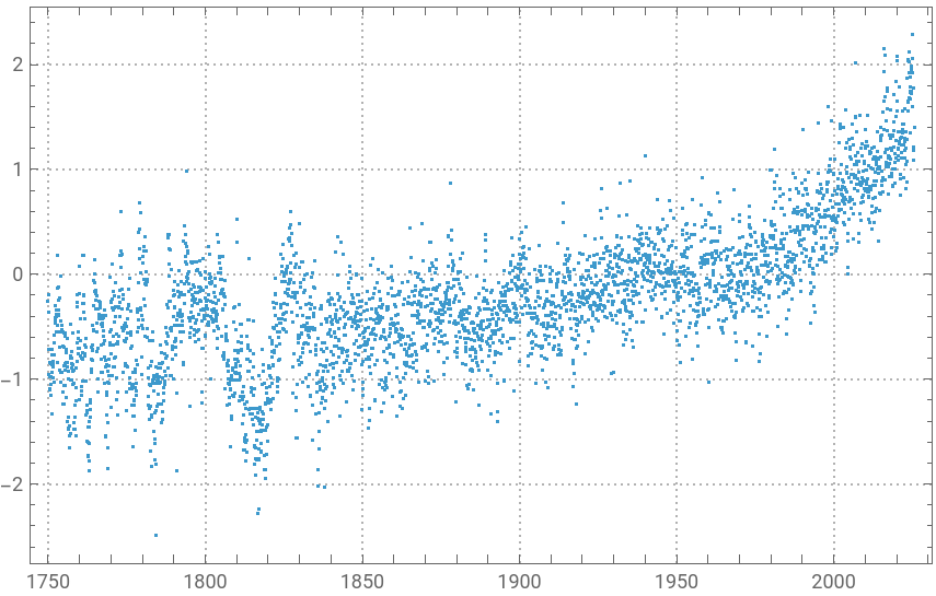
To analyze temperature changes annually, we shift the time series data for each year, aligning them to a common starting point in 1750. This approach allows us to compare temperature changes across different years directly.
In[]:=
dataPRT=ParallelTable[TimeSeriesShift[TimeSeriesWindow[data,DateObject[{y},"Year"]],{1750-y,"Year"}],{y,1750,2024}];
In[]:=
Length[dataPRT]
Out[]=
275
We calculate a rescaled annual mean temperature anomaly for each year and plot these values. This visualization helps us identify overall trends and changes in global temperature patterns over the centuries.
In[]:=
annu=Rescale[Mean/@dataPRT];ListPlot[annu,PlotTheme->"Detailed"]
Out[]=
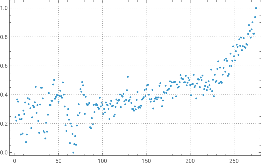
Building the visualization and animation
Building the visualization and animation
Now, we define plotting options for two different types of plots. The first set of options () customizes the appearance of the temperature anomaly plots, including colors and styles. The second set () adjusts the style for individual year plots, ensuring consistency in visualization.
plot1OPT
plot2OPT
In our animated visualization, we use to create an interactive display of global temperature anomalies from 1750 to 2024. The animation highlights each year sequentially, showing how temperature anomalies have evolved over time. The header and subtitles provide context, emphasizing significant temperature records and the period covered.
In[]:=
ClearAll[plot1OPT,plot2OPT];plot1OPT[k_]:={ImageSize->600,AspectRatio->1,PlotStyle->Directive[.6,Thickness[.002]],DateTicksFormat->{"MonthNameShort"},Background->Black,BaseStyle->15,FrameStyle->GrayLevel[.85],PlotRange->{Automatic,{-2.1,2.4}},InterpolationOrder->2,PerformanceGoal->"Speed",ColorFunctionScalingFalse,ColorFunction->(Opacity[(1-3.5#(1-#))^.7&@Rescale[#2,.5lohi],ColorData["TemperatureMap"][Abs[(2+#2)/3.5]^2]]&),Epilog->Text[Style[1749+k,50,ColorData["TemperatureMap"][annu[[k]]]],Scaled[{.5,.98}],{Center,Top}]};plot2OPT={PlotStyle->Directive[Opacity[1],Thickness[.01]],InterpolationOrder->2,PerformanceGoal->"Speed",ColorFunctionScalingFalse,ColorFunction->(ColorData["TemperatureMap"][Abs[(2+#2)/3.5]^2]&)};head=Style["2024 Warmest Year on Record",GrayLevel[.8],40,FontFamily->"DIN Condensed"];header=Style["Global Temperature Anomalies 1750–2024",GrayLevel[.8],25,FontFamily->"Arial Narrow"];sub=Style["Land-surface air monthly °C deviations from 1951–1980 average",GrayLevel[.8],15,FontFamily->"Arial Narrow"];Manipulate[Framed[Column[{head,Style["",.1],header,sub,Show[DateListPlot[dataPRT[[;;k]],plot1OPT[k]],DateListPlot[dataPRT[[k]],plot2OPT]]},Alignment->Center],Background->Black,FrameMargins15],{{k,Length[dataPRT]},1,Length[dataPRT],1},SaveDefinitions->True]
Out[]=


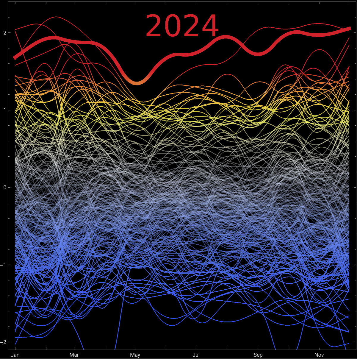
Finally, we export the animation as a GIF, specifying display durations for different frames to control the animation speed. This step allows us to share the dynamic visualization with others, showcasing the changes in global temperature anomalies over the covered period.
CITE THIS NOTEBOOK
CITE THIS NOTEBOOK
2024 was the warmest on record: Global Temperature Anomalies 1750-2024, land-surface air monthly °C
by Vitaliy Kaurov
Wolfram Community, STAFF PICKS, October 2, 2025
https://community.wolfram.com/groups/-/m/t/3554064
by Vitaliy Kaurov
Wolfram Community, STAFF PICKS, October 2, 2025
https://community.wolfram.com/groups/-/m/t/3554064