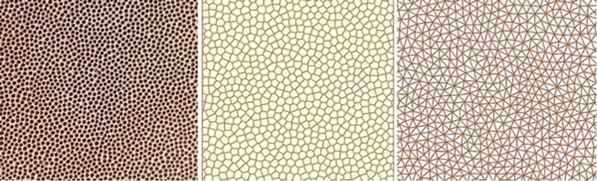
Nature is an inexhaustible source of ideas for mathematicians. I was interested in the structure of pores some mushrooms, which looks very "geometrical". And at first sight can be easily explained.In fact, it was not easy to model it. Here is a possible and convincing method, which also allows to generate a lot of different nature-like structures
Previous approaches
Previous approaches
Poisson disk + Lloyd relaxation
Poisson disk + Lloyd relaxation
In previous post, was proposed an algorithm for the distribution of points on area, that gave results very similar to the distribution of pores. Both visually and statistically. It is based on Poisson disk sampling with the following few steps of Lloyd relaxation. But such approach is purely descriptive. It reproduces the result well, but obviously the mushroom pores do not arise as a selection of random samples.
Turing patterns as PDES solution
Turing patterns as PDES solution
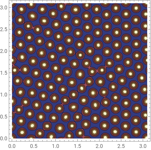
I was told that these structures are very similar to Turing patterns, that are often found in the nature. A simple model is known, consisting of only two PDEs and four parameters, which implements the chemical process that leads to the formation of such structures. This model is implemented in Wolfram Documentation. I wrote my code, and with the given parameters we get patterns that are very similar to pores picture.
Clear[solTuring];solTuring[(*Diffusionparameters*)du_,dv_,(*Reactionparameters*)f_,k_,(*Maxtime*)T_,(*Gridsize*)size_]:=Module[{u,v,t,x,y,eqs,bndConds,initConds,initReg,rndInit,sol},eqs={D[u[t,x,y],t]==duLaplacian[u[t,x,y],{x,y}]-u[t,x,y]*v[t,x,y]^2+f(1-u[t,x,y]),D[v[t,x,y],t]==dvLaplacian[v[t,x,y],{x,y}]+u[t,x,y]*v[t,x,y]^2-(f+k)v[t,x,y]};bndConds={u[t,0.,y]==u[t,size,y],u[t,x,0.]==u[t,x,size],v[t,0.,y]==v[t,size,y],v[t,x,0.]==v[t,x,size]};initReg=0.16size<x<0.96size&&0.16size<y<0.96size;rndInit[c_,r_,s_,num_,initReg_,def_]:=Interpolation[Flatten[Table[{x,y,Piecewise[{{RandomReal[{c+r,c-r}],initReg}},def]},{x,0,s,s/num},{y,0,s,s/num}],1],InterpolationOrder->0];initConds={u[0.,x,y]==rndInit[0.5,0.05,size,100,initReg,1.][x,y],v[0.,x,y]==rndInit[0.25,0.05,size,100,initReg,0.][x,y]};sol=Quiet@NDSolve[Join[eqs,bndConds,initConds],{u,v},{t,0,T},{x,0.,size},{y,0.,size},Method->{"MethodOfLines","SpatialDiscretization"->{"TensorProductGrid","MaxPoints"->100,"MinPoints"->100,"DifferenceOrder"->2}}];{u,v}/.First@sol];
Next evaluation takes ~10 sec on general PC
In[]:=
res=solTuring[0.00031,0.000047,0.03,0.0635,20000,3.1]
Result:
In[]:=
ContourPlot[res[[2]][19900,x,y],{x,0,3.1},{y,0,3.1},PlotRange->All,Contours->6]
Out[]=
However, there are problems:
◼
The resulting structure is very strongly and sharply dependent on the values of the parameters.
Both the parameters of the equation system itself and the settings of the solution method.
It is very difficult to explore the options.
Both the parameters of the equation system itself and the settings of the solution method.
It is very difficult to explore the options.
◼
I don’t know how to get thousands of pores for statistics in a reasonable time
◼
This system is a mathematical model of chemical reaction. Although biochemistry is certainly relevant to the formation of pores, in fact their formation - process in biological tissue, defined by cell division, fabric elasticity, etc.
Cellular automata
Cellular automata
Here is proposed the implementation of the algorithm from the article as a cellular automaton. Unfortunately, it also works long enough and is sensitive to parameters. I tried to get Turing patterns with classical CA, but so far without success. Maybe later it will work.
Relaxation in potential
Relaxation in potential
Definition of potential
Definition of potential
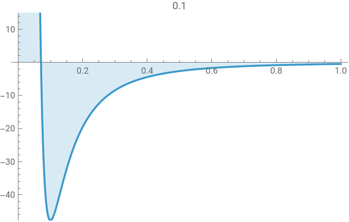
Among many others, the model of pores as particles interacting with a certain potential energy proved to be very suitable. The form of potential must take into account that biological tissue resists both compression and stretching. The analysis of real pores shows that there is a certain average distance at which they stabilize. This fact describes well the classical two-power potential
U(r)=α+
p
1
r
p
2
r
If the following conditions are satisfied:
p
1
p
2
p
2
α
p
1
than we have energy minimum in
r
min
1
p
1
p
2
-
p
2
α
p
1
And conversely, if we set the desired average distance δ between pores and powers of potential, we can calculate the appropriate coefficient:
α=--
p
2
p
1
p
2
p
1
δ
In[]:=
Clear[energy,coreDist,getCoeff];energy[pt_,pts_,α_,pow1_,pow2_]:=Total[(α+)&/@(EuclideanDistance[pt,#]&/@pts)];coreDist[α_,p1_,p2_]:=If!PossibleZeroQ@p1&&!PossibleZeroQ@p2&&p1>p2&&p2αp1<0,,None;getCoeff[δ_,p1_,p2_]:=If!PossibleZeroQ@p1&&!PossibleZeroQ@p2&&p1>p2,,None;
pow1
#
pow2
#
1
p1-p2
-p2
αp1
-p2
p1
p2-p1
δ
Clear[a,p1,p2,d];Manipulatea=getCoeff[d,p1,p2];PanelIfNumberQ@a,Plota+,{x,0,1},PlotRange->{a+,15},Filling->Axis,PlotLabel->d,PlotHighlighting->None,Style["Invalid parameters",Bold,13],ImageSize->{300,250},{{p1,-2.8},-5.,5.,0.01},{{p2,-2.95},-5.,5.,0.01},{{d,0.1},0.001,0.5,0.001},{{a,{}},ControlType->None},SaveDefinitions->True
p1
x
p2
x
p1
d
p2
d
Out[]=


Relaxation method
Relaxation method
In serious studies of many particle systems, complex, smart algorithms are used. Some of them are optional with the built-in NMinimize. But first of all, I doubt that mushrooms use anything like this =)
Second, it requires a lot of computing resources.
I stopped at the simplest, natural approach:
In the small disk surrounding each pore, select a small number of samples and pore moves to a point that realizes the minimum potential energy among them.
Second, it requires a lot of computing resources.
I stopped at the simplest, natural approach:
In the small disk surrounding each pore, select a small number of samples and pore moves to a point that realizes the minimum potential energy among them.
Additional considerations
Additional considerations
Pores are not given immediately, in full quantity. They appear as the fungus grows in those places where there is not yet. And of course there is no long-range interaction. The relaxation of their positions occurs as a result of an elastic reaction of the mushroom tissue between adjacent pores. To obtain more natural results, we perform several steps of relaxation between the birth of new pores.
Final module
Final module
Graphics
Graphics
Evaluation
Evaluation
We start with a small number of randomly distributed pores:
If possible, it is advisable to run parallel computations:
Set parameters and validation.
Input format:
{"Number of neighbors",
"Number of test samples",
"Radius of disk for samples",
"Supposed average distance",
"First energy power",
"Second energy power",
"Rate of new pores per step",
"Number of relaxation steps"}
Input format:
{"Number of neighbors",
"Number of test samples",
"Radius of disk for samples",
"Supposed average distance",
"First energy power",
"Second energy power",
"Rate of new pores per step",
"Number of relaxation steps"}
It is better to carry out iterations in small portions, so you can plan your calculation time (on average for 6 cores the first 20 iterations takes ~10 sec, but with increasing number of pores time grows). And change the parameters on the fly, getting even more interesting results.
Some examples
Some examples
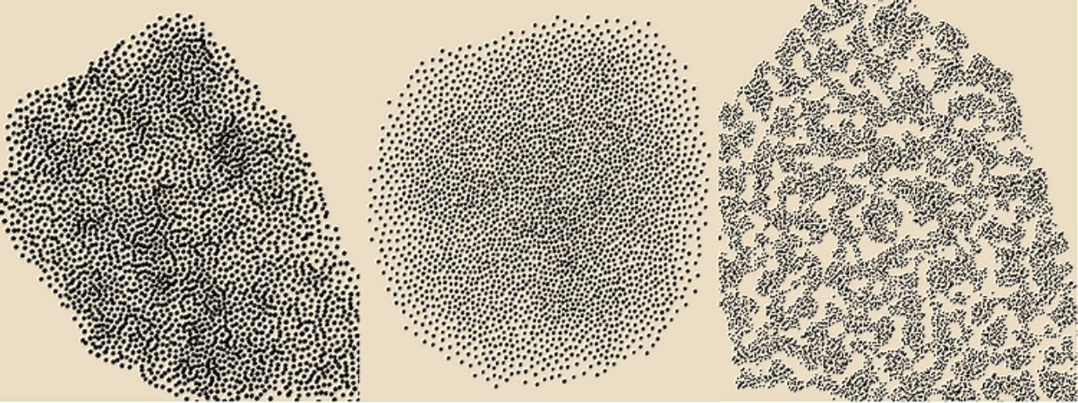
By changing parameters (including during iterations) you can get a huge number of different structures. It is important that the dependence on parameters is not critical and patterns smoothly pass from one to another.
◼
Preset 1
Typical tinder polypore pattern
Typical tinder polypore pattern
◼
Preset 2
◼
Preset 3
◼
Preset 4
Frequently observed Turing patterns
Frequently observed Turing patterns
◼
Preset 5
CITE THIS NOTEBOOK
CITE THIS NOTEBOOK
Fungi pores pattern: final approach
by Denis Ivanov
Wolfram Community, STAFF PICKS, June 17, 2025
https://community.wolfram.com/groups/-/m/t/3480611
by Denis Ivanov
Wolfram Community, STAFF PICKS, June 17, 2025
https://community.wolfram.com/groups/-/m/t/3480611