In this essay, we elaborate on the Period-String Length Law and establish it's credibility through self-collected data from a pendulum physics experiment. We also delve into a more complicated problem of having two pendulums (a coupled system) instead of a single pendulum and look at the nature of synchronization between pendulums. Synchronization in nature is practically everywhere, from neurons synchronizing in epileptic reactions or natural energy being harnessed from industrial synchronizing pendulums.
Introduction
Introduction
We can accredit the creation of the pendulum clock to Christaan Huygens, or The Father of the Pendulum Clock. Clocks in Huygens's time lost 15 minutes a day while Huygen's pendulum clocks would lose merely 15 seconds a day. How did he come up with such a brilliant invention? In the early 1600s, Galileo was experimenting with pendulums and found a useful property in pendulums that made them a good timekeeper: isochronism. This is simply that the period of the swing changes based on string length.
Normally, we know this relation as where T is the period, l is the string length, and g is the gravitational constant. We can verify this relation with some data.
Normally, we know this relation as
T2π
l
gstart=-π/2;θ=start+Pi/6;f[s_Circle]:=s/.Circle[a_,r_,{start_,end_}]({s,Arrow[{#-r/10^6{-Sin@end,Cos@end},#}]}&[a+r{Cos@end,Sin@end}])arc=Graphics@f[Circle[{0,0},1,{-Pi/2,-1.0}]];polygon=Polygon[{{-1,0},{1,0},{1,1/4},{-1,1/4}}];top=Graphics[{Gray,polygon}];circle1=Graphics[Circle[{0,-1/20},1/20]];circle2=Graphics[Circle[{2,-3},1/5]];circle3=Graphics[{Dashed,Circle[{0,0},3.6,{-1.57,-1.0}]}];line1=Graphics[{Dashed,Line[{{0,-1/20},{0,-3.8}}]}];line2=Graphics[{Thick,Line[{{0.03,-0.07},{1.9,-2.83}}]}];arrow=Graphics[{Red,Arrowheads[0.08],Arrow[{{1.986,-3.0},{1.986,-4.6}}]}];line3=Graphics[{Line[{{2.2,-3.8},{2.9,-3.8}}]}];arrow2a=Graphics[{Arrowheads[0.04],Arrow[{{0.7,-3.8},{0,-3.8}}]}];arrow2b=Graphics[{Arrowheads[0.04],Arrow[{{1.3,-3.8},{1.98,-3.8}}]}];text1=Graphics[Text[Style["L sinθ",FontSize14,Purple],{1.0,-3.8}]];text2=Graphics[Text[Style["mg",FontSize14,Purple],{2.1,-4.8}]];line3=Graphics[{Line[{{1.0,-3.6},{2.9,-3.6}}]}];line4=Graphics[{Line[{{2.2,-3.0},{2.9,-3.0}}]}];text3=Graphics[Text[Style["L(1 - cosθ)",FontSize14,Purple],{2.7,-3.3}]];arrow3a=Graphics[{Arrowheads[0.04],Arrow[{{2.6,-3.35},{2.6,-3.6}}]}];arrow3b=Graphics[{Arrowheads[0.04],Arrow[{{2.6,-3.27},{2.6,-3.0}}]}];text4=Graphics[Text[Style["L",FontSize14,Purple],{1.2,-1.5}]];text5=Graphics[Text[Style["θ",FontSize16,Purple],{0.2,-0.7}]];text6=Graphics[Text[Style["O",FontSize14,Purple],{-0.16,-0.2}]];textT=Graphics[Text[Style["T",FontSize14,Black],{1.15,-2.1}]];arrowT=Graphics[{Blue,Arrowheads[0.08],Arrow[{{1.88,-2.8},{1.2,-1.8}}]}];Show[top,circle1,circle2,circle3,line1,line2,line3,arrow,arrow2a,arrow2b,text1,text2,line4,text3,arrow3a,arrow3b,text4,text5,text6,arrowT,textT,arc]
Out[]=
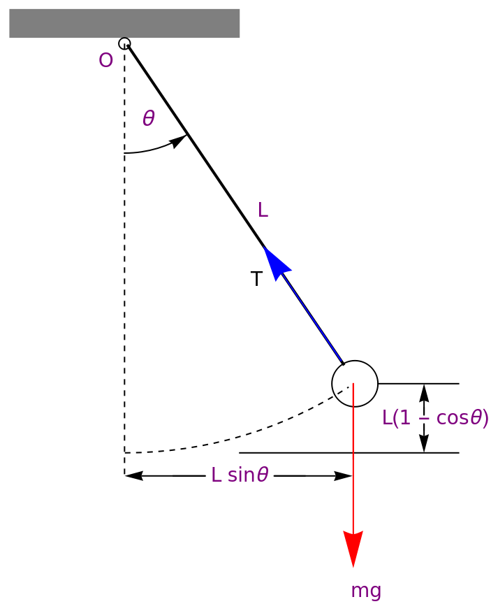
The above diagram is a classical pendulum and is the type of pendulum that we will be referencing to for the rest of this article. We notice that the diagram includes the weight of the pendulum bob (mg), the tension force pointed upwards along the rope (T), the string length (L), and the angle relative to the vertical and pivot (θ). The code is quite messy but it creates a wonderful diagram.
Period-String Length Relation
Period-String Length Relation
In[]:=
Insert[Grid[{{StringLength,T1,T2,T3,T4,Average},{26.4,1.09,1.13,1.08,1.06,Mean[{1.09,1.13,1.08,1.06}]},{35.4,1.33,1.27,1.32,1.25,Mean[{1.33,1.27,1.32,1.25}]},{38.7,1.33,1.36,1.41,1.33,Mean[{1.33,1.36,1.41,1.33}]},{46.6,1.46,1.40,1.34,1.45,Mean[{1.46,1.40,1.34,1.45}]},{52.2,1.64,1.57,1.56,1.55,Mean[{1.64,1.57,1.56,1.55}]}},Frameall],{DividersAll,Spacings1.5{1,1}},2]
Out[]=
LengthString | T1 | T2 | T3 | T4 | Average |
26.4 | 1.09 | 1.13 | 1.08 | 1.06 | 1.09 |
35.4 | 1.33 | 1.27 | 1.32 | 1.25 | 1.2925 |
38.7 | 1.33 | 1.36 | 1.41 | 1.33 | 1.3575 |
46.6 | 1.46 | 1.4 | 1.34 | 1.45 | 1.4125 |
52.2 | 1.64 | 1.57 | 1.56 | 1.55 | 1.58 |
◼
The String Length is in Centimeters (cm) and the trial times are all in seconds (s).
◼
We can derive the period-string length relation from the data above, we just graph the squared averages. Why squared? Keep reading.
In[]:=
data={{26.4,1.1881},{35.4,1.67056},{38.7,1.84281},{46.6,1.995156},{52.5,2.2964}};line=Fit[data,{1,x},x]Show[ListPlot[data,PlotStyleRed],Plot[{line},{x,0,52.5}]]
Out[]=
0.196853+0.0401241x
Out[]=
We have placed the line of best fit for the data table above, and a linear fit seems to be pretty good. We can find the approximate slope of the line from the coordinates (26.4, 2.29) and (52.2, 1.181). So = 4.29.From arranging 4.024. Hey! That's pretty close to 4.29. Thus, we verified the string length-period relationship. The experimental data is pretty close to the actual constant, with a relatively small experimental error. This could be due to air currents or inconsistences in the letting-go of the pendulum, human error, etc.
2.29-1.181
0.522-0.264
2
T
l
4
2
(π)
g
Synchronizing Pendulums
Synchronizing Pendulums
Once Huygens made his pendulums, he decided to ply around with them. When he was sick in bed, he sat two pendulums next to each other and let them swing at different speeds and different initial angles. Eventually, after a while, they synchronized their motion. Meaning, that they were moving with the exact same speed at the exact same angle. There are two types of synchronization....
◼
In Phase Synchronization: The speed and angle of the pendulums are exactly at all times during the synchronization period.
◼
Anti Phase Synchronization: The speed of the pendulums are exactly the same at all times during the synchronization period. Although, their motions are directly opposite of each other.
A big question is, what even causes this synchronization? Well, let's start with the equation of motion of a pendulum. We will utilize Lagrangian physics here. We can find the Euler Lagrange solutions to find the equations of motion and graph them to see if anything cool happens! The technical terminology isn't too important here as much as the visual representations are. We can look at the graph below...
L(M+2m)()+ml(cos()+cos())+m++mgl(cos()+cos())-k
1
2
2
x
x
θ
1
θ
1
θ
2
θ
2
2
l
2
θ
1
2
θ
2
θ
1
θ
2
1
2
2
x
In[]:=
sol=NDSolve[{30x''[t]+y''[t]Cos[y[t]]+z''[t]Cos[z[t]]-y'[t]^2Sin[y[t]]-z'[t]^2Sin[z[t]]+30x[t]+2x'[t]==0,y''[t]+x''[t]Cos[y[t]]+Sin[y[t]]-x'[t]y'[t]Sin[y[t]]+0.02y'[t]==0,z''[t]+x''[t]Cos[z[t]]+Sin[z[t]]-x'[t]z'[t]Sin[z[t]]+0.02z'[t]==0,x[0]==0,x'[0]==0,y[0]==Pi/10,y'[0]==0,z[0.5]==1,z'[2]==0},{x,y,z},{t,0,1000}]Plot[{Evaluate[y[t]/.sol],Evaluate[z[t]/.sol]},{t,0,250},PlotRangeAll]
Out[]=
xInterpolatingFunction,yInterpolatingFunction,zInterpolatingFunction


What does this graph even mean? In short, if these are the equations of motion of the pendulums, then the graph represents the synchronization of the pendulums. We notice that as the value on the x-axis gets larger, the graph thins out and the curves are almost perfectly opposite of each other. This is a result of damping. This may be friction on the floor, between the pivots, on the bob and string, etc. But, this graph proves that for there to be synchronization, there needs to be damping on the system, otherwise synchronization will not occur.
To look at how the string length of a pendulum affects the synchronization time of pendulums in a coupled system, take a look at the following article: https://doi.org/10.36227/techrxiv.24492313.v1.
There is still a lot of research to be done with synchronizing pendulums, but it's great to work on! In fact, that's what a lot of my research is about.
References
References
Kukkapalli, N. (2023, November 9). Temporal analysis of synchronizing coupled pendulums based on varying string lengths. figshare. https://www.techrxiv.org/articles/preprint/Temporal_Analysis_of_Synchronizing_Coupled_Pendulums_based_on_Varying_String_Lengths/24492313
Russell, D. (2018, June 8). Acoustics and Vibration Animations. Oscillation of a Simple Pendulum. https://www.acs.psu.edu/drussell/Demos/Pendulum/Pendulum.html
Morin, D. (n.d.). The Lagrangian Method - Scholars at Harvard. Harvard University. https://scholar.harvard.edu/files/david-morin/files/cmchap6.pdf
CITE THIS NOTEBOOK
CITE THIS NOTEBOOK
Temporal Analysis of Classical Pendulums: Synchronization and Other Laws
by Niyathi Kukkapalli
Wolfram Community, STAFF PICKS, November 13, 2023
https://community.wolfram.com/groups/-/m/t/3064094
by Niyathi Kukkapalli
Wolfram Community, STAFF PICKS, November 13, 2023
https://community.wolfram.com/groups/-/m/t/3064094