ABSTRACT (original article): MINFLUX is an emerging super-resolution technology that measures the position of single fluorophores with nanometer precision using fewer photons than any other fluorescence imaging or tracking technique. Here, we derive simple and instructive analytical equations for MINFLUX localization precision with a special focus on background photons. A fluorescence background, either arising from an imperfect zero of the MINFLUX excitation point spread function (PSF) or from auto- or out-of-focus fluorescence, ultimately limits the resolution achievable with MINFLUX. Building on previous work, we try to improve our understanding of the influence of background, especially when it is unknown, through a new set of expressions for the localization precision, based on an explicit background term instead of signal-to-background ratio. We use these equations to generate an intuitive understanding of how fluorescence background affects MINFLUX measurements and illustrate that:
- The precision of an emitter position estimate depends on the gradient of its excitation profile.
- Knowledge of the fluorescence background, obtained during post-processing of MINFLUX traces or through separate measurements, provides a better localization precision than in the case of unknown background.
- In diffraction-limited systems, localization with a PSF that features a near-zero minimum outperforms localization with a maximum.
We also present an analytical expression for the localization precision in orbital tracking, which we use for comparison to MINFLUX. CITATION (original article): Zach Marin, Jonas Ries (2024), Approximations of MINFLUX Localization Precision with Background. arXiv:2410.12427. https://doi.org/10.48550/arXiv.2410.12427
The goal here is to understand the influence of background on MINFLUX precision. We follow the framework in Masullo et al. Biophys. Rep. 2022 (and in Yvan Eilers’ thesis) to construct CRLB estimates for MINFLUX measurements using quadratic functions in 1D.
Localization of emitters in 1D
Localization of emitters in 1D
Minimum
Minimum
For MINFLUX excitation, let’s consider a quadratic equation
In[]:=
f
quad
σ
q
The first order approximation of localization precision is
In[]:=
dx
0,quad
f
quad
f
quad
Out[]=
x0
2
N
Minimum with known background
Minimum with known background
Now let’s consider a quadratic measured at x=-L/2, L/2 in the case of a known background value.
In[]:=
p0=[-L/2];p1=[L/2];psum=p0+p1;p0n=p0/psum;p1n=p1/psum;=FullSimplifySqrt1N*p0n+p1n,{b>0,N>0,L>0,>0}
f
quad
f
quad
σ
minK2sb
2
D[p0n,x0]
2
D[p1n,x0]
σ
q
Out[]=
1
4
2
+4+8b
2
L
2
x0
2
σ
q
2
(-4)
2
L
2
x0
2
σ
q
2
L
2
x0
2
σ
q
2
L
2
-4+8b
2
L
2
x0
2
σ
q
For b = 0, this simplifies to
In[]:=
σ
minK2sbb0
σ
minK2sb
Out[]=
2
L
2
x0
4L
N
Which is equivalent to S22b in the Balzarotti 2017 paper supplement...
In[]:=
FullSimplify(1+)-,{N>0,L>0,x0<L}
L
4Sqrt[N]
2
(x0/(L/2))
σ
minK2sbb0
Out[]=
0
For x0 = 0 we obtain
In[]:=
σ
minK2sbx0
σ
minK2sb
σ
q
Out[]=
2
L
2
σ
q
4L
N
And at x0=0, b=0, we get the standard equation (S22c in Balzarotti 2017)...
In[]:=
σ
minK2sbb0x0
σ
minK2sbb0
Out[]=
L
4
N
And if we evaluate the simple single-measurement first order approximation at =L/2, we obtain the same result:
x
0
In[]:=
dx
0,quad
Out[]=
L
4
N
Now let’s consider a quadratic measured at x=-L/2, 0, L/2 in the case of a known background value.
In[]:=
p0=[-L/2];p1=[L/2];p2=[0];psum=p0+p1+p2;p0n=p0/psum;p1n=p1/psum;p2n=p2/psum;=FullSimplifySqrt1N*p0n+p1n+p2n,{b>0,N>0,L>0,>0}
f
quad
f
quad
f
quad
σ
minK3sb
2
D[p0n,x0]
2
D[p1n,x0]
2
D[p2n,x0]
σ
q
Out[]=
+2b+16b+4+4b
2
x0
2
σ
q
2
+6+12b
2
L
2
x0
2
σ
q
2
(-4)
2
L
2
x0
2
σ
q
2
L
2
x0
2
σ
q
2
L
2
x0
2
(-4)
2
L
2
x0
2
σ
q
4
L
2
L
2
x0
4
x0
2
σ
q
2
L
2
x0
2
σ
q
2
2
For =0, this simplifies to
x
0
In[]:=
FullSimplify[/.x0->0,{>0,N>0,L>0}]
σ
minK3sb
σ
q
Out[]=
1
4
+8b+12b
2
L
2
σ
q
2
L
2
σ
q
2
L
Because this is a case of known background, we can directly substitute values in the definition to compute the SBR at b=0.01:
In[]:=
SBR
x
0
σ
q
Out[]=
1.33333
Minimum with unknown background
Minimum with unknown background
Now let’s consider the K=3 case with unknown background.
In[]:=
p0mat={{D[p0n,x0]^2,D[p0n,x0]*D[p0n,b]},{D[p0n,b]*D[p0n,x0],D[p0n,b]^2}};p1mat={{D[p1n,x0]^2,D[p1n,x0]*D[p1n,b]},{D[p1n,b]*D[p1n,x0],D[p1n,b]^2}};p2mat={{D[p2n,x0]^2,D[p2n,x0]*D[p2n,b]},{D[p2n,b]*D[p2n,x0],D[p2n,b]^2}};J=FullSimplify[N*((1/p0n)*p0mat+(1/p1n)*p1mat+(1/p2n)*p2mat)];invJ=FullSimplify[Inverse[J],{L>0,A>0,b>0}];=FullSimplify[Sqrt[invJ[[1,1]]]]
σ
minK3
Out[]=
1
4
+6+12b-12+192+8b(+48)
2
L
2
x0
2
σ
q
4
L
2
L
2
x0
4
x0
2
L
2
x0
2
σ
q
4
L
Now let’s make substitutions.
In[]:=
σ
minK3s
σ
minK3
x
L
b
L
σ
q
σ
q
σ
q
Out[]=
1
4
(1+12+6)(1+8+12(-1+32)+192)
b
L
2
x
L
b
L
b
L
2
x
L
4
x
L
N
For =0 this simplifies to
x
0
In[]:=
FullSimplify[/.x0->0,{>0,N>0,L>0}]
σ
minK3
σ
q
Out[]=
1
4
+8b+12b
2
L
2
σ
q
2
L
2
σ
q
2
L
which matches the known case.
Now let’s plot a comparison of the unknown and known backgrounds.
In[]:=
xx={L->50,->250,b->0.01,N->100};Plot{/.xx,/.xx},{x0,0,25},PlotStyle->{Blue,Red},PlotLegends->Placed[{"b known","b unknown"},{Left,Top}],PlotRange->{{0,25},{0,20}},FrameLabel->" (nm)",None,{" (nm)",None},Frame->{{True,False},{True,False}},LabelStyle->{FontSize->14,FontFamily->"Arial"}
σ
q
σ
minK3sb
σ
minK3
σ
x
0
x
0
Out[]=
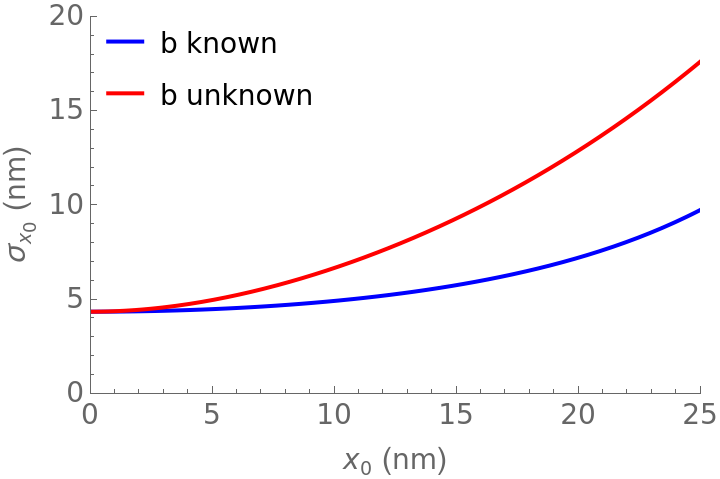
Localization precision in the presence of different background sources
Localization precision in the presence of different background sources
K=2
K=2
Let’s consider the =0 case. We can convert b and N to background photons Nb and signal photons Nb by making the observation that Nb=2Ab and ^22+^22.
x
0
A=
N
s
2
(L/2-x0)
σ
q
2
(L/2+x0)
σ
q
In[]:=
σ
minK2sbNsNb
σ
minK2sb
N
b
σ
q
σ
q
N
s
N
b
N
s
N
b
N
s
Out[]=
L+
N
b
N
s
4
N
s
In the first instance, let’s consider the case where background comes from a non-perfect 0. In this case, Ntot = Ns.
In[]:=
σ
minK2sbimperfect
σ
minK2sb
N
s
σ
q
N
s
Out[]=
2
L
2
σ
q
4L
N
s
Now let’s consider the case where background comes from out-of-focus fluorescence. In this case, we have to find the contribution from Ns and Nb.
K=3
K=3
In the first instance, let’s consider the case where background comes from a non-perfect 0. In this case, Ntot = Ns.
Now let’s consider the case where background comes from out-of-focus fluorescence. In this case, we have to find the contribution from Ns and Nb.
Maximum
Maximum
Suppose we use the Gaussian function to approximate the Airy maxima
The first order approximation of the localization precision is
We can compare this to the minimum approximation:
Maximum with a known background
Maximum with a known background
Let’s consider the negative quadratic equation, an expansion of the 1D Gaussian.
For x0=0 this simplifies to
For x0=0 and no background we get:
Now let’s consider the Gaussian case.
At x0=0, this becomes
Let’s plot this as a function of b and L.
At b = 0, this becomes
This is equivalent to S23b in Balzarotti 2017 in the event you swap his definition of a Gaussian with ours...namely 4*Log[2] becomes (1/2)...
And at x0=0, b=0, this is again in agreement with S24b in Balzarotti 2017 if you swap 1/(4*Log[2]) for 2...
This is the same as the simple single measurement approximation evaluated at -L/2
Comparison of minima and maxima
Comparison of minima and maxima
First, let’s do a quick comparison of the K=2 cases for the maximums and minimum evaluated in the presence of background.
Now, let’s do the main text figures.
Localization of emitters in 2D
Localization of emitters in 2D
First, a 1D donut for sanity
First, a 1D donut for sanity
OK, this matches equation S22f in the Balzarotti 2017 supplement.
2D MINFLUX with known background
2D MINFLUX with known background
Let’s construct a donut following the definition in Eilers Section 2.1, but add a background term.
And compute the localization precision
Let’s confirm this matches Balzarotti S27...
...hooray!
Now let’s check the equivalence to Balzarotti 2017 S31, which is computed with SBR...
And we see this indeed matches S31 with a change of variables.
Orbital tracking
Orbital tracking
Let’s try constructing orbital tracking measured at only three evenly distributed points on a circle.
Let’s plot this as a function of L and b.
CITE THIS NOTEBOOK
CITE THIS NOTEBOOK
Approximations of MINFLUX localization precision with background
by Zach Marin & Jonas Ries
Wolfram Community, STAFF PICKS, November 6, 2024
https://community.wolfram.com/groups/-/m/t/3315725
by Zach Marin & Jonas Ries
Wolfram Community, STAFF PICKS, November 6, 2024
https://community.wolfram.com/groups/-/m/t/3315725