We begin by considering some novel approaches to the construction of metamathematical space. By requiring proof paths to behave in a particular way, we obtain a structure alternative to the current picture of entailment cones (nevertheless highly dependent on it). We establish connection between metamathematical space and the category theory. Toy example of category is constructed.
Part 1: Metamathematical spacetime
Part 1: Metamathematical spacetime
in which we explore the paths of truth
What is metamathematical space? What mathematical properties should it capture? In this section we explore this question by studying automated theorem proving systems.
To clarify. By automated theorem proving (ATP), I don't mean what is usually meant by it in the literature. Instead, I consider sort of automated theorem generators. You can think of it as ATPs that attempt to prove every possible theorem from the axioms, asymptotically generating the space of all true theorems.
Automated theorem proving and proof paths – motivation for a new picture
Automated theorem proving and proof paths – motivation for a new picture
Let’s begin with the non-accumulative entailment structure consisting of theorems as its vertices, with edges being rewritings of theorems according to the fixed set of axioms, like this one:
In[]:=
g=[{x<->y,y->z},x↔y,4,GraphLayoutAutomatic,AspectRatio1/3,ImageSizeScaled[.6]]
Out[]=
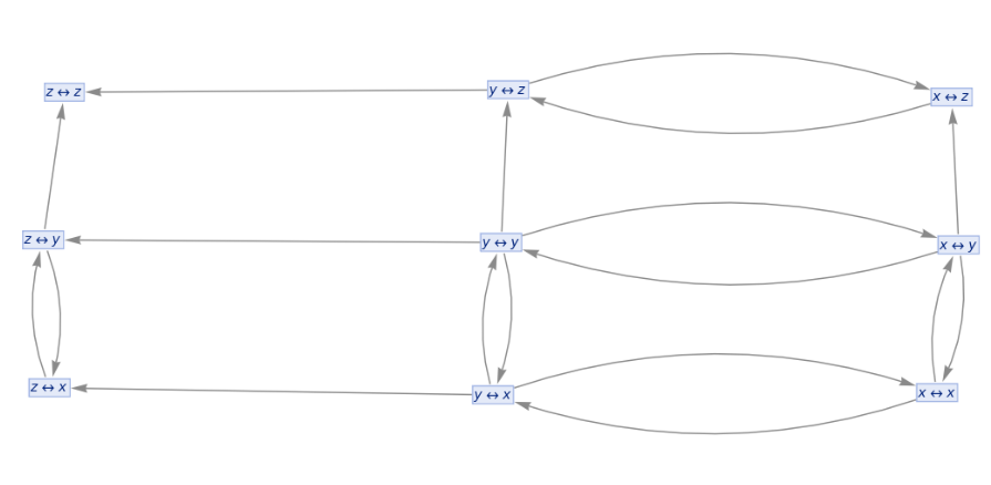
If we wanted to construct a particular proof, say prove from , this proof would be just a path in this space:
z<->x
x<->y
In[]:=
HighlightGraphg,StylePathGraph[FindShortestPath[g,x↔y,z↔x],DirectedEdges->True],["ProofPathStyle"]
Out[]=
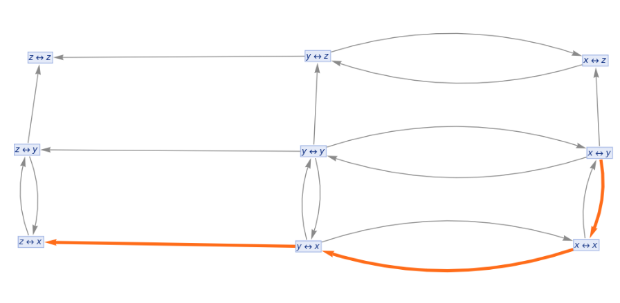
Now let us consider a number of ATPs working in parallel, starting from the same initial condition and proving theorems at random. Again, they try to achieve from . Then, one prover can – for example – go straight to the end, whereas the other be stuck in some loop for a while, using up more computational resources before it terminates. (One could argue that going around in loops could be avoided, as no reasonable ATP would do that, but, in general, the question of whether or not one is in a loop is computationally irreducible until one finally gets out. And to even know if one’s out, a big enough memory is needed). How can we express this relative dynamics on standard entailment graph? It turns out we can’t. This picture lacks a dynamical aspect of ATPs. It does not capture the amount of computational resources used during the proving process. From this point of view, proof paths in this space are analogous to trajectories in space in the physics case, not relativistic worldlines through spacetime. What we were calling entailment structure, or even entailment cones, now seems to be rather a purely spatial construct. Entailment structures seem like richer versions of branchial graphs, with differences and properties that we will discuss further down the text. As we progress, the spacelike-ness of entailment structures will become even more apparent. For that reason, from now on I won’t use the terms like “entailment cone”, and start referring to entailment structure as “metamathematical space”, as opposed to “metamathematical spacetime”, which I’ll introduce in the next paragraph.
z<->x
x<->y
So how can we construct what might be called the proper analogue of spacetime in the case of metamathematics? We will do this by knitting together all possible worldlines of our ATPs. In time step 0, we start from our initial theorem (), and every ATP is in that state. In time step 1, there are three possible states our ATPs can move to, so we will put them on the next time slice and make causal connections between them and our initial theorem at time slice 0. There is one caveat, however. Should we be able not to move? That is, to progress through time, but not through space? It is certainly possible in physics, one can just choose not to move. In metamathematics, there is one more interpretation of this process of not moving: on the semantic level, every theorem entails itself. Thus, truly random ATP can in principle just be using up resources on proving identity on every step. Doing this has yet another property: every theorem you ever proved on every time slice is present on next slices. This fact that will come in handy later. For these reasons, we will include these “identity events” in the picture of metamathematical spacetime; you can just go perfectly well without them if you prefer. Next is the picture of metamathematical spacetime built from these principles. The one that correctly captures relative dynamics of theorem provers, and the one in which “entailment cones” are actual spacetime light cones.
x<->y
In[]:=
Out[]=
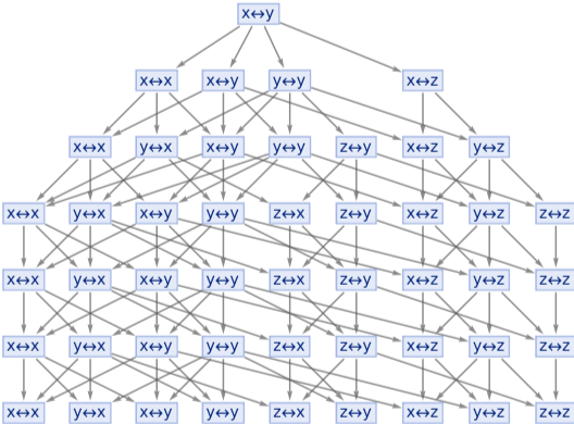
This picture captures all possible relations between ATPs starting from the same initial state and working in parallel. One can see all possible proof paths and their interactions. We can see that there are effectively three event horizons contained within each other. If ATP proves any theorem that is beyond any of these event horizons, it can never come back to the theorems on the left. In this case, it seems pretty excessive to continue this evolution. As evolution settles down, there is no new information involved. But something similar can happen in physics, too. For example, think about heat death and the universe in thermodynamic equilibrium. However, thermodynamic equilibrium requires sort of coarse-graining of spacetime to happen. But as we see in the next section, this is exactly what we are doing in the case of metamathematics.
Some properties of metamathematical space(time)
Some properties of metamathematical space(time)
Although we managed to establish close connections between physics and metamathematics, there are still some significant differences between physical and metamathematical space(time)s. The reason for these differences lies essentially in different scales at which we probe what we call the points of our space. In the physics project, we operate at the level of structureless emes. This in effect prevents us from having things like absolute points in space, because the emes just appear and disappear constantly. There is no way of ascribing prevailing time existence to emes. In the case of mathematics as explored in this project, however, we operate at the levels of whole theorems, and we think of our metamathematical space as basically labelled points. This labelling and fact that theorems prevail through time allow us to build the picture of “spacetime” like the one above, something that would be impossible in the case of physics. At this level, metamathematical spacetime seems more Newtonian than Einsteinian. Points of this coarse-grained space have distinct labels and conserve their identity through time. To find analogies with the physics project, it would be desirable to eliminate that property. The labelling can be thought of as analogous to the particular coordinatization of physical space. This suggests that perhaps the very statement of a theorem can be observer-dependent. Observers in different reference frames would collect different sets of emes into theorems and coordinatize their space differently. But at the level of this project, we are left with Newton-esque spacetime and work within one particular coordinate system. (As said, that property is what allows us to even construct something like the metamathematical spacetime. At the level of emes, such concept would be ill-defined, as it is the case with physics, and we could only work with full multiway graphs – what we will nevertheless do in the next section, where we consider accumulative systems).
Multiway graphs for metamathematical space
Multiway graphs for metamathematical space
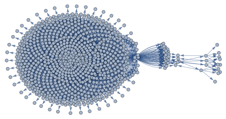
Until now, we essentially studied a particular type of ATPs, namely the ATPs with constant memory complexity, which can know only the initial and final state and the sets of axioms. Therefore, we could only move from one theorem to another using one of our axioms. The only possible moves were the random ones, as we didn’t know where we had already been. What if wanted to consider a somewhat more realistic ATP, that is the one that has some nontrivial memory complexity and, in turn, is able to optimize the proving process. What are the properties of such ATP? Firstly, it can store already proven theorems in the memory and use them as lemmas to prove other theorems. Secondly, it will not waste computational resources for proving already proven theorem, unless it encounters it again during proving from newly generated theorems. In other words, it will never repeat the exact same proof. How can we implement those features, how can we represent multiple such ATPs working in parallel? At any given step, any possible state of our ATPs consists of all of the theorems proven so far and all the proofs used to do so. It is just regular entailment structure! The possible states of these ATPs are all possible entailment structures one can obtain from a given initial structure (usually set of unconnected “axioms”). What are the steps ATPs can follow? Essentially, every elementary step is just one new proof that can occur in an entailment structure. Each proof consists of one theorem to be proved from, and the other used as a rule to be updated with. Effectively, what we get is a kind of a multiway token-event graph, where each path consists of a series of consecutive one-proof extensions of the initial structure, and one considers all the paths at once. Here is an example of such structure:
In[]:=
example=SimpleGraphCatenate@Rest@NestListgraphs|->Catenate@Mapgraph|->graphGraph[VertexList[graph],Join[EdgeList[graph],#]]&/@CatenateApplyKeyValueMap{k,r}|->#1r,#2r,CanonicalizePatterns@*First/@ResourceFunction["MultiReplace"][#1,makeReplaceRule@@#2,(*Method->"Bisubstitution",*)Heads->False]&/@Tuples[VertexList[graph],{2}],graphs/._g_:>g,{Graph[{a_∘(b_∘c_)<->(a_∘b_)∘c_,a_∘1<->a_},{}]},2,VertexShapeFunction->_:>(Inset[Framed[SimpleGraph[#2,ImageSize->15]],#1,#3]&),GraphLayout->"LayeredDigraphEmbedding",PerformanceGoal->"Quality",AspectRatio->14//VertexReplace[#,g_:>Sort@EdgeList[g]]&
k
k
Out[]=
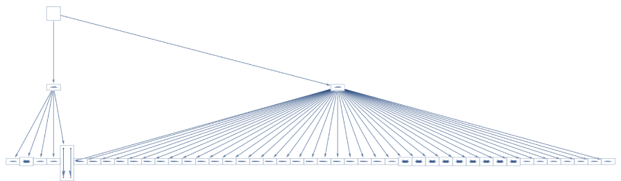
Here in different rendering, evolved for one more step:
In[]:=
examplealt=SimpleGraphCatenate@Rest@NestListgraphs|->Catenate@Mapgraph|->graphGraph[VertexList[graph],Join[EdgeList[graph],#]]&/@CatenateApplyKeyValueMap{k,r}|->#1r,#2r,CanonicalizePatterns@*First/@ResourceFunction["MultiReplace"][#1,makeReplaceRule@@#2,Method->"Substitution",Heads->False]&/@Tuples[VertexList[graph],{2}],graphs/._g_:>g,{Graph[{a_∘(b_∘c_)<->(a_∘b_)∘c_,a_∘1<->a_},{}]},3,(*VertexShapeFunction->_:>(Inset[Framed[SimpleGraph[#2,ImageSize->1]],#1,#3]&),*)GraphLayout->"SpringElectricalEmbedding",PerformanceGoal->"Quality",AspectRatio->12//VertexReplace[#,g_:>{Sort@VertexList[g],Sort@EdgeList[g]}]&
k
k
Out[]=
Part 2: Dream of Categorification
Part 2: Dream of Categorification
in which we learn the meaning of “meaning”
Now, when we have developed a different picture of metamathematical spacetime, we will study possible connections between metamathematics and category theory and ponder over extracting semantics from syntax.
When I’m writing that something is correct for “categories”, I don’t really mean all categories. I mean some subclass of them. I was only be able to look into really toy examples of some finite categories of groups, so you can treat all my statements about categories as applicable only to them. The ideas are yet to be formalized, but in the end I expect that some generalized version of the method will work at least for some sort of algebraic or concrete categories.
General remarks on categorical properties
General remarks on categorical properties
Where should we start looking for an emerging behavior of categories from the structure of theorem space? We can get the initial idea from the foundational book on metamathematics, where we extract group elements from the expressions space using “droplets”. Group elements are just equivalence classes of expressions under the relation of being equivalent in a given set of axioms, with group action as appending chosen representative of a given class. Can we do something similar in the case of all categories, can we somehow extract the objects and morphisms as we extracted the Cayley graph of the group? Well, almost. The first observation will be that now don’t want to deal with expressions and start from some arbitrary collection, we want to deal with purely accumulative structures of theorems. So maybe we can do something similar and treat collections of theorems as distinct groups? I found this approach right, because what is a particular group if not the set of theorems it satisfies? But there are significant differences compared to the droplet case. The firsts one is that the groups won’t be these separate droplets generated by the equivalence classes, because every group have to at least satisfy group axioms, so they all intersect. The second one is what really this sets of theorems represent. Let’s focus on the group case and consider the set of bare group axioms. What object of the category of groups it represents? We can immediately see that it does not represent an object, a particular group, but rather all possible free groups. All free objects are the ones that are characterized by satisfying exactly the group axioms and nothing more. And this will be the case for all other sets of axioms. They do not represent distinct groups, but rather equivalence classes of groups modulo free groups under the free product operation. Here, we will sweep this problem under the carpet by considering the category of subgroups of some finite group, so the only free object will be the trivial group.
Construction of a category
Construction of a category
Let us now proceed to the process of extracting known categorical semantics (in the terms of objects and morphisms) from purely syntactical data about theorems. We will start with (not necessarily minimal) set of axioms for the Klein group. Using standard presentation of the group, these becomes:
As we want to study the category of groups, we will divide this set into two subsets: the group axioms, which every object must satisfy and which define the category, and “object axioms”, which will be used to construct individual objects:
Let us now generate multiway entailment structure for all of these axioms:
Here is how it looks like in different rendering:
We can imagine that different possible subgroups correspond to different possible set of axioms that they satisfy. Therefore, let’s highlight theorems derived from different possible subsets of our axioms system:
Where the label indicates what axioms were not used in proving process. Let’s now draw the relations of inclusion between this subgraphs. They will correspond to monomorphisms in our category.
If one looks carefully at what these red figures represents, one discovers that left down corner behaves like trivial group, top right is the Klein group, and the other two are different encodings of the two-element group.
Concluding remarks
Concluding remarks
We generated different objects in our category by looking at different subsets of theorems they may satisfy. By doing that, we provided external data to our model. Would it be possible to extract the information about objects purely from the structure of the graph? Is it somehow encoded in its automorphisms?
Keywords
Keywords
◼
Metamathematics
◼
Causality
◼
Categories
Acknowledgment
Acknowledgment
It was a joy to write this. In the end, I went a bit literary and had a good fun with titles. Big, big thanks to James Boyd for being an amazing mentor and also to Nik Murzin – saying that he helped with the code would be an understatement.
References
References