Introduction
Introduction
On September 8, 2026, OpenAI announced that an internal AI system had produced a solution to the Navier–Stokes existence and smoothness Millennium Prize Problem [1-2].
The construction produces a smooth fluid flow that, under a carefully designed force field, develops into an increasingly intense vortex spiraling inward toward the origin. As the vortex core shrinks, its velocity grows, ultimately producing a singularity in finite time. The velocity, pressure, nonlinear transport, and viscous terms all become large in a precisely coordinated way, so that the Navier-Stokes equations continue to hold point by point throughout the flow, while the required external force remains smooth and finite [3].
The complete proof is extremely intricate and spans more than 150 pages [3]. In this post, we will instead try to build an intuitive picture of the underlying mechanism using simplified mathematics and Wolfram Language visualizations.
The Navier Stokes Equation
The Navier Stokes Equation
The Navier–Stokes equation is essentially Newton's second law, , applied to a moving fluid. Instead of following a single object, we describe a velocity field , which tells us the velocity of the fluid at every point in space and time. For an incompressible Newtonian fluid, the equation can be written as [4]
F=ma
u(x,t)
∂u
∂t
1
ρ
2
∇
together with the incompressibility condition
∇·u=0
Imagine standing on a bridge and watching a river. The term measures whether the water at a fixed point is speeding up or slowing down with time. The nonlinear term describes the fact that moving water carries its motion with it, so fast water flowing into a slower region can change the velocity there. The pressure-gradient term, , pushes water from higher pressure toward lower pressure. The viscous term, tends to smooth velocity differences between neighboring parts of the fluid, much like friction between neighboring layers of fluid [4].
∂u
∂t
(u·∇)u
∇p
νu
2
∇
The force represents any additional external influence, such as a pump or wind. Finally, expresses incompressibility: water cannot simply pile up or disappear. If a river narrows, the water must speed up so that the amount flowing in still matches the amount flowing out [4].
f
∇·u=0
A useful way to read the equation is therefore: the acceleration of a small fluid parcel must be exactly balanced by pressure, viscosity and external forcing. The equation is local. This balance must hold at every point and at every time.
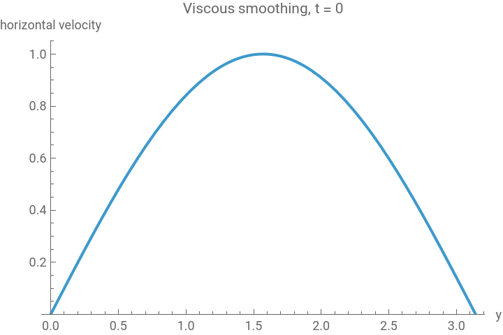
As an example, take a two-dimensional shear flow of the form . Because the horizontal velocity depends only on , the incompressibility condition is automatic and the nonlinear transport term vanishes. With constant pressure, the Navier–Stokes equation reduces exactly to the one-dimensional diffusion equation [4]
u=(v(y,t),0)
y
(u·∇)u
∂v
∂t
2
∂
∂
2
y
Suppose the fluid initially has the profile between two stationary walls at and . The walls enforce zero velocity there. NDSolveValue can evolve the profile directly [5]:
sin(y)
y=0
y=π
In[]:=
Clear[v,y,t];ν=.1;vsol=NDSolveValue[{D[v[y,t],t]==νD[v[y,t],{y,2}],v[y,0]==Sin[y],v[0,t]==0,v[Pi,t]==0},v,{y,0,Pi},{t,0,6}];ManipulatePlotvsol[y,t0],{y,0,Pi},,{t0,0,6},
Out[]=


In simple flows, only a few terms dominate and exact solutions are possible. In complicated three-dimensional flows, however, nonlinear transport, pressure, viscosity and vortex stretching interact across many spatial scales. These interactions allow the same equation to describe smooth laminar motion, vortices and turbulence, while also making its mathematical analysis remarkably difficult [4].
The Millennium Prize Problem
The Millennium Prize Problem
In 2000 the Clay Mathematics Institute selected the Navier–Stokes existence and smoothness problem as one of the seven Millennium Prize Problems, with a prize of one million US dollars for a correct solution. The mathematical question is whether the three-dimensional equations always continue to describe a smooth velocity field when they start from smooth, physically reasonable initial data, or whether the dynamics can concentrate motion so strongly that a singularity forms in finite time [2].
What exactly has to be proved?
What exactly has to be proved?
Consider the three-dimensional incompressible Navier–Stokes initial-value problem
∂u ∂t 1 ρ 2 ∇ |
∇·u=0 |
u(x,0)= u 0 |
For smooth divergence-free initial data, a smooth solution is known to exist for at least a short time. The mystery is what happens later. Does the solution remain smooth for every future time, no matter how complicated the flow becomes? Or can some quantity become unbounded at a finite time , so that the classical solution cannot be continued? The official Clay formulation allows either direction: prove global existence and smoothness (A, B in [2]), or exhibit a mathematically valid breakdown scenario satisfying the stated hypotheses (C, D in [2]).
T
Why is the problem so difficult?
Why is the problem so difficult?
Even ordinary three-dimensional flows are already difficult to solve exactly. The velocity has three interacting components, pressure is coupled to the whole flow, and the nonlinear term continually mixes different directions and scales. Closed-form analytic solutions therefore exist only for rather special geometries or symmetries. For a general 3D flow, the Navier–Stokes equation must nevertheless be satisfied at every point in space and at every instant of time [4].
This pointwise requirement makes constructing a singularity especially delicate. If we were allowed to apply a force that itself became infinite, producing an infinite velocity would not be very surprising: the singularity could simply be coming from the external forcing. The interesting challenge is to start with a force field that remains smooth and finite, yet arrange the internal fluid motion so that the velocity becomes singular on its own [2-3].
Pressure also makes the problem more subtle. In an incompressible fluid, pressure adjusts throughout the flow to maintain . A small intense vortex is therefore not completely isolated: through pressure, it can interact with the rest of the fluid [4].
∇·u=0
Finally, numerical simulation cannot by itself settle the Millennium Problem. A computation can certainly detect and resolve very intense behavior, including a developing singularity, as long as the relevant spatial and temporal scales remain larger than the numerical resolution. The difficulty is proving that the observed growth continues all the way to a true mathematical singularity rather than eventually being regularized at still smaller scales. Conversely, an apparent blow-up may change when the grid is refined. Numerical experiments can therefore provide strong evidence and insight, but a proof must control the continuum equations at arbitrarily small scales [2, 4].
What has already been tried and achieved?
What has already been tried and achieved?
Leray showed that three-dimensional Navier–Stokes flows have global weak solutions [6], so the equations do not simply stop making mathematical sense after some finite time. The difficulty is that a weak solution is allowed to be much rougher than an ordinary smooth velocity field. Since then, mathematicians have found many conditions that guarantee smoothness: sufficiently small initial flows remain smooth, and a solution cannot become singular unless certain measures of its velocity or vorticity become extremely large [4, 7].
Partial-regularity results go further and show that, if singularities occur at all, they must be confined to an extraordinarily small part of space-time [8].
In other words, decades of work have placed a very tight fence around any possible singularity, but have not yet proved that the fenced-in possibility is empty.
What would a successful solution have to accomplish?
What would a successful solution have to accomplish?
A proof of global regularity would need to identify a mechanism that prevents indefinite concentration at every possible scale. In practical terms, one would like a scale-critical quantity that is controlled for all time, or a structural argument showing that vortex stretching necessarily weakens before it can outrun viscosity. A proof of breakdown would have to do the opposite: construct a genuine Navier–Stokes flow in which concentration repeatedly reinforces itself, overcomes diffusion and all pressure/nonlinear cancellations, and reaches a mathematically demonstrable singularity in finite time [2-3, 7].
OpenAI's Approach - Simplified
OpenAI's Approach - Simplified
The full OpenAI construction is technically very elaborate. The central idea is to construct a velocity field that becomes singular in finite time, arrange the large terms in the Navier–Stokes equation to cancel each other, and then prove that the external force left over after this cancellation is completely smooth [3].
Basic Approach
Basic Approach
For the breakdown route used by OpenAI, the target is to construct a smooth external force together with a smooth incompressible flow that starts from rest, has finite kinetic energy, and nevertheless develops unbounded velocity at a finite time. OpenAI normalizes the singular time to . If we already have a divergence-free velocity field and a pressure , we can formally solve the Navier–Stokes equation for the required force [2-3]:
t=1
u
p
f=+(u·∇)u-νu+∇p
∂u
∂t
2
∇
In that sense, the construction can be viewed as working backwards. Instead of first specifying a force and asking what flow it creates, we try to design the singular flow we want and then compute the force required to support it. But this observation by itself proves almost nothing: an arbitrary singular velocity field will usually produce a singular force. The real achievement is to engineer and so carefully that the large and potentially divergent pieces of the residual cancel, leaving a force that remains smooth, together with all of its derivatives, even at the singular time [3].
u
p
The construction can be pictured as three connected regions:
i. At the center is a shrinking, rapidly spinning vortex that produces the blow-up.
ii. Around it is an annular transition region containing carefully designed oscillatory pulses; these supply the momentum transport missing from the background vortex.
iii. Farther out is a smooth exterior flow whose speed decreases with radius and which can ultimately be cut off in space.
The core creates the singularity, the annulus repairs the momentum balance, and the exterior makes the whole construction compatible with a smooth localized force [3].
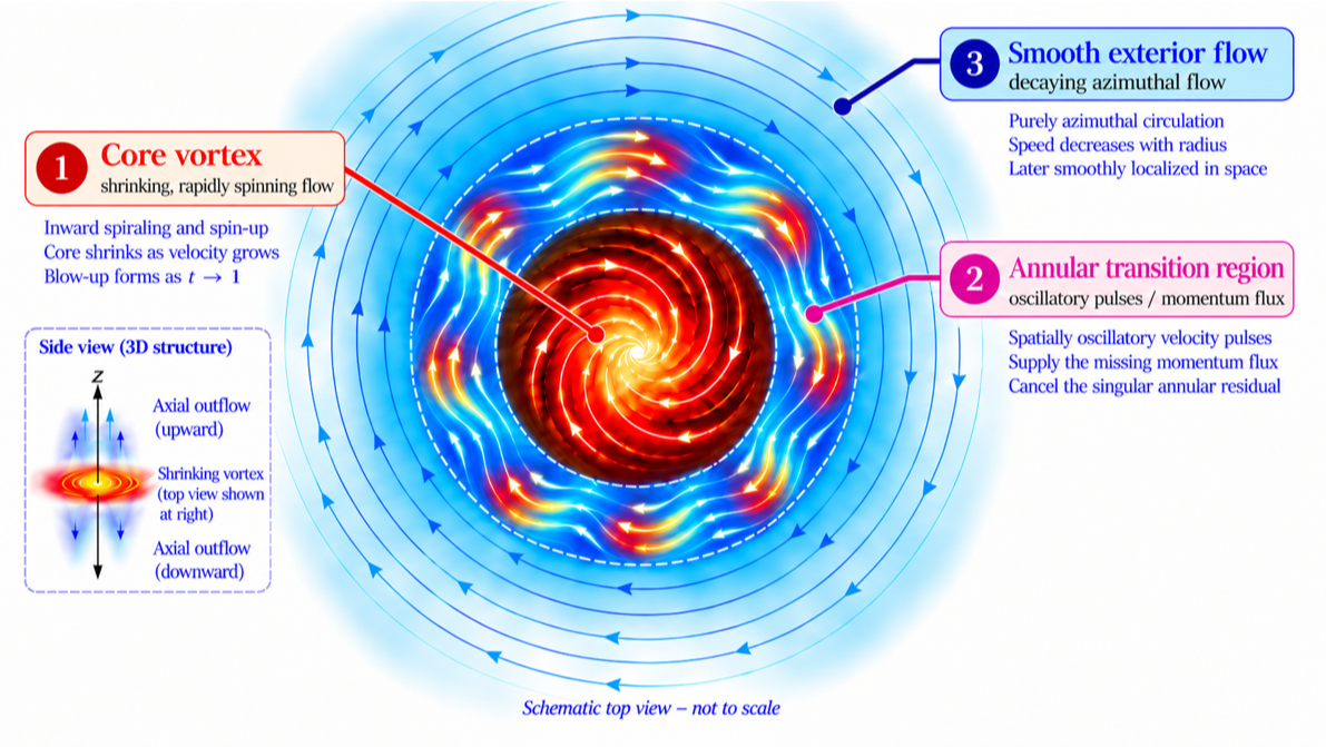
Figure 1: Schematic of the three-region Navier–Stokes blow-up construction: a shrinking core vortex, an oscillatory transition annulus, and a smooth decaying exterior flow [3].
It is useful to see this backwards viewpoint directly in Wolfram Language. The following helper computes the Navier–Stokes residual of a proposed velocity and pressure field. If the field were an exact unforced solution, this residual would be zero; otherwise it is precisely the force that would have to be supplied.
Clear[navierStokesResidual];navierStokesResidual[u_,p_,vars_,t_,nu_]:=Simplify[D[u,t]+Grad[u,vars].u-nu(Laplacian[#,vars]&/@u)+Grad[p,vars]]
Now take a deliberately simple blowing-up vortex: rigid rotation whose angular speed grows like . A quadratic pressure exactly balances the centripetal part of the nonlinear acceleration.
-
1
2
(1-t)
In[]:=
Clear[x,y,z,t,a];a[t_]:=(1-t)^(-1/2);uToy={-a[t]y,a[t]x,0};pToy=1/2a[t]^2(x^2+y^2);FullSimplify[{Div[uToy,{x,y,z}],navierStokesResidual[uToy,pToy,{x,y,z},t,nu]},0<=t<1]
Out[]=
0,-,,0
y
2
3/2
(1-t)
x
2
3/2
(1-t)
The Core Vortex
The Core Vortex
Both scales go to zero, but the radial scale shrinks slightly faster than the axial scale. The intense part of the vortex therefore becomes thinner and thinner compared with its height: a rapidly concentrating slender column around the origin [3].
At the same time the velocity grows. The characteristic scales in the OpenAI construction are
This is one of the most striking features of the construction: the maximum speed goes to infinity while the kinetic energy of the concentrating core actually tends to zero [3].
Here is an animation based on approximate equations that illustrates how the concentrating vortex core becomes increasingly slender in rescaled coordinates:
Animation 1: A concentrating core in rescaled coordinates, revealing increasing axial-to-radial aspect ratio
The scaling estimate can be checked symbolically. The first factor below is the radial cross-sectional area, the second is the axial length, and the last is the squared characteristic velocity.
Thus, in this simplified scaling model, the core energy tends to zero even while the characteristic velocity tends to infinity.
A useful simplified way to represent the self-similar structure is to introduce rescaled coordinates
and then think schematically of the central profiles as
Why can such a rapidly growing flow still satisfy Navier–Stokes? Because the leading terms grow at matching rates. For example, in the azimuthal equation the time variation, radial transport, axial transport and radial viscous diffusion all have the same characteristic size:
The common scaling of these apparently different terms is easy to verify algebraically:
The profile functions are chosen so that the coefficients of these large terms cancel to leading order. The pressure participates in the same balancing act. In particular, the radial pressure gradient supplies the centripetal acceleration required by the swirl, approximately
while incompressibility ties the inward radial motion to the axial outflow:
So the core should not be pictured as an arbitrary vortex that happens to become large. Its radial inflow, swirl, axial motion and pressure are designed together so that the strongest singular pieces of the Navier–Stokes equation balance locally. The full proof then adds higher-order corrections to make this balance increasingly accurate [3].
The Annular Region
The Annular Region
The core cannot simply continue unchanged to arbitrarily large radius. The final flow must have finite energy, fit smoothly into a well-behaved exterior, and eventually be localized in space. Therefore the singular inner vortex has to transition to a weaker outer flow. This transition takes place in an annular region surrounding the core [3].
Then over many oscillations
Here is an animation based on approximate equations that illustrates the oscillatory radial flow in the annulus, with alternating inward and outward motion around the core:
Animation 2: Alternating inward (teal) and outward (amber) radial flow around the core
This averaging mechanism is especially transparent computationally. Averaging one complete oscillation gives:
The individual oscillatory velocities average to zero, while the products do not. We can go one step further and shift the phase of one component:
Thus there may be almost no net oscillatory velocity, but there can still be a directed transport of angular and axial momentum. OpenAI chooses the amplitudes, orientations and locations of the pulses so that the divergence of these averaged quadratic momentum fluxes supplies precisely the leading contribution missing from the background momentum balance. Schematically, [3]
This is the intuitive purpose of the wavy annular flow. It is not a global cancellation in which an infinite amount of momentum at the core is somehow canceled by another infinity far away. Navier–Stokes remains a local equation. The oscillatory pulses are placed exactly where the background transition has a momentum imbalance, and their nonlinear momentum transport is engineered to cancel that imbalance there. The full proof then adds further corrections so that not only the leading singular term, but the remaining residual and all of its derivatives, become smooth [3].
The Exterior Flow
The Exterior Flow
There is one more useful piece of the picture. Beyond the annulus the flow is chosen to be purely azimuthal and independent of height: the fluid simply circles the axis, with the speed decreasing with radius. Its azimuthal velocity is chosen to satisfy the radial viscous heat equation [3]
Putting the Picture Together
Putting the Picture Together
The simplified mechanism can therefore be summarized as follows. The core is a self-similar vortex whose radius and height shrink while its swirl and axial speed grow without bound. Its leading velocity and pressure profiles are chosen so that the dominant Navier–Stokes terms balance inside the core. The core must then be connected to a harmless exterior, but that transition creates a singular momentum mismatch. Oscillatory pulses in the annulus generate a nonzero mean quadratic momentum flux and are tuned to cancel this mismatch. Finally, higher-order corrections and spatial localization make the remaining residual smooth. The external force is not what directly contains the singularity; rather, the singular behavior is produced by the fluid motion while the force obtained from the final residual remains smooth [3].
This last point is the heart of the result. Designing a velocity field that blows up is easy if one is allowed to apply a force that also blows up. What is difficult is arranging a genuine Navier–Stokes momentum balance in which the velocity becomes unbounded but
extends smoothly through the singular time. OpenAI's proof establishes this much stronger statement, controlling every space-time derivative of the residual [3].
The formulas above should be read as a simplified map of the mechanism, not as a substitute for the detailed profile construction and correction scheme in the paper [3].
Verification
Verification
Although the announced result is extremely promising, it has not yet completed the formal process required for recognition as a solution to a Millennium Prize Problem. The Clay Mathematics Institute has deliberately strict rules: a proposed solution must first be published in a qualifying mathematical outlet, at least two years must normally pass after publication, and the work must achieve general acceptance within the global mathematics community. Only after this period of independent scrutiny does Clay undertake its own detailed evaluation. For now, therefore, it is most accurate to describe the Navier–Stokes problem as having an announced or proposed solution that still awaits full verification and formal recognition.
Clay itself has said that the problem has “apparently been settled,” while emphasizing that its evaluation process is deliberately unhurried and that further updates will follow.
Implications
Implications
Another implication is that the Navier–Stokes equations can, at least mathematically, drive their own continuum description to failure. The construction starts with a smooth velocity field and a smooth, finite external force. Nothing singular is inserted by hand. Nevertheless, the internal dynamics concentrate the motion into a smaller and smaller region until the velocity becomes unbounded in finite time. In that sense, the continuum model creates a state that the classical continuum model itself can no longer describe. This does not mean that a real fluid would literally acquire infinite velocity. Navier–Stokes treats matter as a continuous medium, but real fluids are made of molecules. As the relevant length scales become extremely small, effects ignored by the continuum model would eventually become important. At that stage one would need a more microscopic description, such as kinetic theory or molecular dynamics [1, 4].
Tristan Buckmaster and the Road to the Solution
Tristan Buckmaster and the Road to the Solution
The OpenAI result did not appear in a vacuum. In the months leading up to the announcement, Tristan Buckmaster of New York University and Levent Alpöge had been pursuing a closely related program for constructing finite-time singularities in fluid equations. Their work built on ideas developed over several years by Diego Córdoba and Luis Martínez-Zoroa, who had introduced a mechanism for producing blow-up using carefully designed forcing. Buckmaster himself has been very explicit that the fundamental idea belongs to Córdoba and Martínez-Zoroa, and that he and Alpöge used modern AI systems to push this program substantially further [9-10].
For most of a year their progress was gradual. Then, on August 15, 2026, Buckmaster and Alpöge obtained finite-time blow-up with smooth forcing for the Boussinesq and three-dimensional Euler equations; the arguments were formally verified in Lean by August 22. They also reported progress on hypodissipative Navier–Stokes. These were not yet a solution of the Millennium Problem, because the ordinary three-dimensional Navier–Stokes equations contain the full viscous term, but they represented a major step toward it [10-11].
The significance of this progress was already clear before OpenAI announced its result. On September 7, Terence Tao wrote that Buckmaster and Alpöge had made enough of a breakthrough that extending the construction to Navier–Stokes appeared “very feasible” in the near future. He described their method as repeatedly adding small, increasingly high-frequency corrections that make the solution more singular while keeping the required forcing smooth. This is strikingly close in spirit to the central difficulty discussed throughout this post: create an ever more violent internal flow while ensuring that the externally applied force itself remains perfectly regular [12].
There is also an unusual historical connection between this work and OpenAI’s announcement. OpenAI states that it began its intensive Millennium Problem effort on September 1 after hearing rumors of major progress, rumors it later understood to be connected with Buckmaster and Alpöge. OpenAI says its system independently completed the Navier–Stokes construction and Lean verification by September 6, and it explicitly recognizes Buckmaster and Alpöge’s priority on their forced-Euler result. OpenAI also states that it did not access their private work and that, following an investigation, their Codex prompts could not have influenced the system used for the result [1].
Buckmaster has presented a different perspective on some aspects of this episode. In his public statement, he emphasized that the smooth-forcing route to the Clay problem was a very specific direction that he and Alpöge had quietly chosen to pursue, and he raised questions about how OpenAI came to work on the same general route shortly after information about their progress began circulating. Importantly, however, Buckmaster explicitly wrote that he did not know whether OpenAI had used any of their data and was “not accusing anyone of anything.” [10]
Whatever one makes of that controversy, I think the scientific contribution deserves to be separated from it. Buckmaster and Alpöge demonstrated that the Córdoba–Martínez-Zoroa program could be pushed much further than previously known, reaching smooth-forced blow-up for the full three-dimensional Euler equations and making the path toward Navier–Stokes much more concrete. Their work also helped bring the relevant mechanism to the attention of the wider mathematical community immediately before the Millennium Problem breakthrough [9-12].
In my view, the community therefore owes real gratitude not only to Tristan Buckmaster and Levent Alpöge, but also to Diego Córdoba and Luis Martínez-Zoroa, whose earlier work created the mathematical route on which these later developments were built. Buckmaster himself has strongly emphasized this point. The eventual Navier–Stokes result is remarkable, but so is the chain of human mathematical insight that made such a route visible in the first place [9-10].
References
References
[1] OpenAI (2026). On the Navier-Stokes Millennium Prize Problem. Announcement, September 8; updated September 10, 2026. Source
[2] C. L. Fefferman (2000). Existence and Smoothness of the Navier-Stokes Equation. Clay Mathematics Institute, official Millennium Prize problem statement; alternatives (A)-(D). Source
[3] OpenAI (2026). Finite Time Blowup for Navier-Stokes. 166-page manuscript. See Theorem 1.1; Sections 2.1 (core), 2.2 (annulus), 2.3 (exterior), 3 (proof outline), and 9-10 (smooth residual and localization). Source
[4] A. J. Majda and A. L. Bertozzi (2002). Vorticity and Incompressible Flow. Cambridge Texts in Applied Mathematics 27, Cambridge University Press. Source
[5] Wolfram Research. NDSolveValue. Wolfram Language & System Documentation Center. Accessed September 14, 2026. Source
[6] J. Leray (1934). Sur le mouvement d'un liquide visqueux emplissant l'espace. Acta Mathematica 63, 193-248. Source
[8] L. Caffarelli, R. Kohn and L. Nirenberg (1982). Partial regularity of suitable weak solutions of the Navier-Stokes equations. Communications on Pure and Applied Mathematics 35(6), 771-831. Source
[10] T. Buckmaster (2026). Public statement on the Alpoge-Buckmaster results and discussions with OpenAI. Four-page statement, September 2026; especially pp. 1 and 3-4. Source
[11] L. Alpoge and T. Buckmaster (2026). Blowup for the Boussinesq Equations with Smooth Forcing. Preprint; especially Sections 1-2 (construction, intellectual background and AI statement). Source
[12] T. Tao (2026). Finite time blowup with smooth forcing term for the incompressible porous medium, Boussinesq, and incompressible Euler equations. What's new, September 7, 2026. Source
CITE THIS NOTEBOOK
CITE THIS NOTEBOOK
An Intuitive exploration of OpenAI's Navier–Stokes singularity construction for the $1M Millennium Prize Problem
by Jayanta Phadikar
Wolfram Community, STAFF PICKS, September 14, 2026
https://community.wolfram.com/t/28013
by Jayanta Phadikar
Wolfram Community, STAFF PICKS, September 14, 2026
https://community.wolfram.com/t/28013