We attempted to incorporate physical differential equations to training of a neural network, so that we may be able to make predictions over a domain larger than the training data domain. The main challenge was “how to use the latest state of the net being trained, take its derivatives, and add those to the loss term.” Many in-built functions, and compositions of in-built functions were tried. Finally, we devised a way to use the the net for building custom loss functions. Next, we will try to tweak and improve the performance of the eventual net.
Analytical Solution to generate our data
Analytical Solution to generate our data
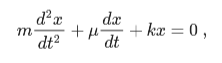
In the first step, we use the already known physics equations to generate training and testing data for our model. The equation for the 1D damped harmonic oscillator is:
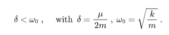
in the underdamped state :
Oscillator function
Oscillator function
This function takes in two parameters δ and , and an x position, and outputs the y position for the same.
ω
0

In[]:=
oscillator[d_,w0_,x_]:=Module[{w,phi,A,cos,exp,y},w=Sqrt[w0^2-d^2];phi=ArcTan[-d/w];A=1/(2*Cos[phi]);cos=Cos[w0*x+phi];exp=Exp[-d*x];y=exp*2*A*cos;y//N]
Generate Data
Generate Data
In[]:=
data=Table[{x,oscillator[2,20,x]},{x,0,0.5,0.01}];traindata=Table[{data[[i]][[1]]}->{data[[i]][[2]]},{i,1,Length[data]}];traindata=RandomChoice[traindata,Length[traindata]];testdata=Table[{data[[i]][[1]]}->{data[[i]][[2]]},{i,1,Length[data]}];testdata=RandomChoice[testdata,Length[testdata]];
Training on a traditional neural network
Training on a traditional neural network
Define a simple net class
Define a simple net class
net function that takes 4 arguments: no. of inputs, outputs, hidden neurons per layer, and number of layers
In[]:=
net[ninput_,noutput_,nhidden_,nlayers_]:=NetChain[{LinearLayer[nhidden],FunctionLayer[Tanh],Table[{LinearLayer[nhidden],Tanh},{nlayers}],LinearLayer[noutput]},"Input"->{ninput}]
Create a net with the required parameters
In[]:=
firstnet=net[1,1,10,2]
Out[]=
NetChain


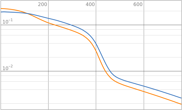
training this net to get a baseline
In[]:=
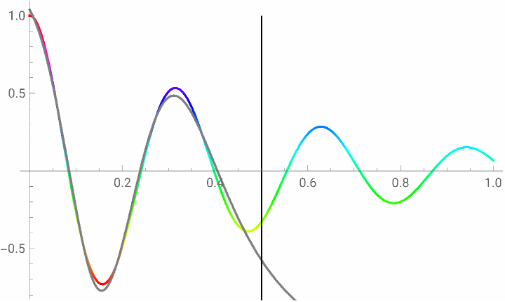
firstnettrained=NetTrain[firstnet,traindata,{"TrainedNet","ResultsObject"},ValidationSettestdata]Show[Plot[oscillator[2,20,x],{x,0,1},ColorFunctionHue],Plot[firstnettrained[[1]][i],{i,0,1},PlotStyle->Gray],Graphics@Line[{{0.5,-1},{0.5,1}}]]
Out[]=
NetChain,NetTrainResultsObject


Out[]=
Structuring the Physics Informed Net
Structuring the Physics Informed Net
To calculate the first and second derivative, we use their formulae derived from first principles :
y’(x)=,andy’’(x)=
lim
h->0
y(x+h)-y(x)
h
lim
h->0
(y(x+2h)-2y(x+h)+f(x))
2
h
To be able to do this, we need to be able to evaluate the latest iteration of the target net, as Wolfram Language doesn’t have an in-built equivalent to AutoGrad.
For doing that, we need to share the parameters from our base model, using the “NetInsertSharedArrays” function, and Initialize the model.
For doing that, we need to share the parameters from our base model, using the “NetInsertSharedArrays” function, and Initialize the model.
In[]:=
secondmodel=net[1,1,10,2]
Out[]=
NetChain
In[]:=
secondmodel=NetInsertSharedArrays[secondmodel]secondmodel=NetInitialize[secondmodel]
Out[]=
NetChain
Out[]=
NetChain
“ploss” is a NetGraph that finds the first and second derivative
In[]:=
ploss=NetGraph[<|"d1"->FunctionLayer[Apply[4*(#1-#2)/10^-4&]],"d2"->FunctionLayer[Apply[(#1-2*#2+#3)/((10^-4)^2)&]],"total"->TotalLayer[],"sum"->SummationLayer[],"scale"->FunctionLayer[Apply[#*400&]]|>,{NetPort["net(x+h)"]->"d1",NetPort["net(x)"]->"d1",NetPort["net(x+2h)"]->"d2",NetPort["net(x+h)"]->"d2",NetPort["net(x)"]->"d2","d1"->"total","d2"->"total","total"->"sum",NetPort["net(x)"]->"scale"->"total"}]
To be able to use “ploss”, we need to give it the relevant inputs, we define “NetPhys”
Concluding remarks
Concluding remarks
While this doesn’t work as well as we had hoped it would, we have made progress in the coding problem this project presented, and have got results a bit better than a plain net. What remains to be done is to train the network over more iterations and test out various tweaks like changing the scaling factors, and weight of the loss terms.
Keywords
Keywords
◼
PINN
◼
Physics
◼
Classical mechanics
◼
Harmonic motion
◼
Machine learning
◼
Neural networks
Acknowledgment
Acknowledgment
My mentor Mr. Julian Laverde, TA Mr. Rahul Sharma and Mr. Mike Yeh were instrumental
References
References