The AdS/CFT correspondence posits an equivalence between a gravitational theory(d+2 dimensional anti-de Sitter spaces) and a lower dimensional non gravitational theory(d+1 dimensional conformal field theory). This duality is solely dependent on the AdS boundary conditions. This project seeks to model the AdS/CFT duality within the Wolfram framework by exploring the effect of the AdS boundary conditions on bulk properties such as dimensionality and curvature. We use causal graphs obtained by sprinkling to represent our bulk space. These graphs have coordinates associated with each vertex which are utilized to demarcate subgraphs forming the “bulk” and “boundary” of this space. We define a tensor network on the boundary to calculate the entanglement entropy and then explore connections to the bulk calculations like Hausdorff dimensionality and Ricci scalar curvature.
Introduction
Introduction
◼
AdS/CFT Correspondence
Developed by Juan Maldacena, AdS/CFT correspondence is a gauge/gravity duality that relates a weakly-coupled gravitational theory in Anti De Sitter Space, which is a higher dimensional spacetime with a negative curvature, to a strongly-coupled quantum field theory living on its boundary. This correspondence allows for the study of strongly coupled quantum field theories, which are difficult to analyze using traditional techniques. One explicit realization of AdS/CFT is the Ryu-Takayanagi conjecture: the entanglement entropy of some region in a CFT corresponds to the area of a minimal surface(Ryu-Takayanagi surface) in the bulk gravity theory. Recent works have focused on describing a tensor network CFT ansatz by extending the ideas from classical AdS/CFT to a discrete spacetime model.
1-2
◼
Tensor Networks
An analogous connection between minimal surfaces and entanglement entropy of states also appears in the context of Tensor Networks which has inspired attempts at tensor network models of AdS/CFT framework. Tensor networks are graphical representations of quantum states or quantum operations using tensors. For the prescription of an AdS/CFT model, they utilize unitary operators and isometries to systematically reduce the degrees of freedom of a quantum field theory or a quantum state on a lower-dimensional boundary. This process, called coarse graining, allows us to study the emergent geometry from the entanglement structure of the quantum state at different length scales.
◼
Entropy Calculation
We will be calculating the Von Neumann entropy in our project. Such entropy calculation requires density matrices associated with the respective quantum states.
Let’s fix a spatial slice of bulk AdS. We can imagine covering this surface with a tensor network where each site represents a quantum state. As we go from the bulk to the boundary, the quantum circuit is coarse grained and we thereby lose “connection” between sites as we approach the boundary. The unitaries and isometries ensure that at any chosen site, only a specific number of sites from previous layers would influence its density matrix. This corresponds to an entropy cone which holds similarity to the causal structure of the underlying AdS geometry. This means, at any given site, we can trace out all the states lying outside the former’s entropy cone. Consequently, the connectivity of the geometry is determined by the connections of the tensor network.
Let’s fix a spatial slice of bulk AdS. We can imagine covering this surface with a tensor network where each site represents a quantum state. As we go from the bulk to the boundary, the quantum circuit is coarse grained and we thereby lose “connection” between sites as we approach the boundary. The unitaries and isometries ensure that at any chosen site, only a specific number of sites from previous layers would influence its density matrix. This corresponds to an entropy cone which holds similarity to the causal structure of the underlying AdS geometry. This means, at any given site, we can trace out all the states lying outside the former’s entropy cone. Consequently, the connectivity of the geometry is determined by the connections of the tensor network.
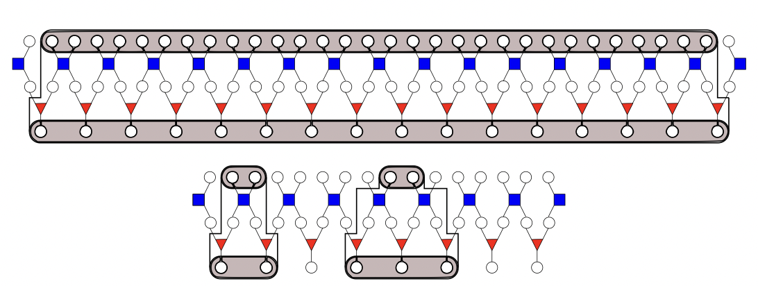
Fig 1 shows the causal cone for one large block of sites after one layer of unitaries and isometries. Once the causal cone reaches a width of one site, the coarse graining terminates.3
Methodology:
Methodology:
1. Causal Graphs:
1. Causal Graphs:
To define the Ryu-Takayanagi surfaces, we first need to define our metric and the corresponding causal structure. We sprinkle random points onto an n-dimensional metric with mass specified as ‘1’ and select only spacelike separated vertices to form our causal graph. The boundary subgraphs are chosen using an optimization function that selects the optimal tolerance value to specify the least distance between a point and the continuum boundary surface for it to lie on the discrete boundary. This tolerance value is of the form:
1/(sprinklepoints)^dimension
where the inverse of the number of sprinkling points is taken to be the discretization scale. Consider the following example of a 7-dimensional Schwarzschild causal structure. The discretization scale is chosen to be 1/300,i.e, we sprinkle 300 random points onto this geometry. Fig 1 shows the causal graph formed by the spacelike separated points. Fig 2 showcases the boundary marked in red over the causal graph. Boundary vertices were chosen as points within _____
◼
GetCausalGraph[dimensions, discretization scale]:=
In[]:=
GetCausalGraph[dim_,discrete_]:=Module[{metric,vertices,phi,causalVertex,Graphs={},boundaryVertices,boundaryGraphs={},space,pair,diff,tuple,edgeList,causalVertices,tupleBoundary,spaceBoundary,causalGraph},metric=MetricTensor[{"HigherSchwarzschild",dim,1}];vertices=Table[{RandomReal[1],RandomReal[1],Table[RandomReal[2*Pi],dim-2]}//Flatten,(1/discrete)];pair=Tuples[vertices,2];pair=Select[pair,!(First[#]==Last[#])&];diff=First[#]-Last[#]&/@pair;space=(metric["LengthPureFunction"][#]^2)/.(Thread[metric["Coordinates"]->#])&/@diff;space=List[#]&/@space;tuple=Join[pair,space,2];causalVertex=Select[tuple,#[[3]]<=0&];causalVertex=Drop[#,{-1}]&/@causalVertex;edgeList=DirectedEdge@@@causalVertex;edgeList=Select[edgeList,First[#][[1]]<Last[#][[1]]&];Graphs=Append[Graphs,SimpleGraph[edgeList]];boundaryGraphs=Append[boundaryGraphs,GetBoundaryGraph[metric,SimpleGraph[edgeList],discrete]];causalGraph=Join[Graphs,boundaryGraphs//Flatten]]
In[]:=
GetBoundaryGraph[metric_,causalGraph_,discrete_]:=Module[{boundaryGraphs={},pair,diff,space,tuple,edgeList,boundaryVertices,causalVertices,lambdaRange,boundary,optimizeLambda},causalVertices=VertexList[causalGraph];pair=Tuples[causalVertices,2];diff=First[#]-Last[#]&/@pair;lambdaRange=Range[1,10,1];space=(metric["LengthPureFunction"][#]^2)/.(Thread[metric["Coordinates"]->#])&/@diff;space=List[#]&/@space;tuple=Join[pair,space,2];Module[{lambda=#},boundaryVertices=Select[tuple,#[[3]]<=0&&#[[3]]>-lambda*discrete&];(*lamda*discretechangesthetolerancevaluetoincludepointsinsideourboundary*)boundaryVertices=Drop[#,{-1}]&/@boundaryVertices;boundaryGraphs=Append[boundaryGraphs,Subgraph[causalGraph,boundaryVertices]]]&/@lambdaRange;boundaryGraphs=List[#]&/@boundaryGraphs;lambdaRange=List[#]&/@lambdaRange;boundary=Join[boundaryGraphs,lambdaRange*discrete,2];optimizeLambda=Optimize[boundary];Select[boundary,MemberQ[optimizeLambda,Last[#]]&]]
Optimize[boundaryGraphs_]:=Module[{thickness={},vertices,lambda,max={},points={},param},Module[{graph=#,ensemble},vertices=VertexList[graph[[1]]];points=Append[points,Length[vertices]];ensemble=Tuples[vertices,2];With[{pair=#},thickness=Append[thickness,Length[FindShortestPath[graph[[1]],First[pair],Last[pair]]]]]&/@ensemble;max=Append[max,Join[TakeLargest[thickness,1],List[graph[[2]]]]]]&/@boundaryGraphs;points=List[#]&/@points;param=Join[max,points,2];TakeSmallestBy[Select[param,0.15*200<=#[[3]]<=0.4*200&],First,1][[All,2]](*Thecriteriaforanoptimalboundarygraphareasfollows:ithastheminimumthicknessandnumberofvertexpointsbetween15%and40%ofthetotalnumberofcausalvertices.*)]
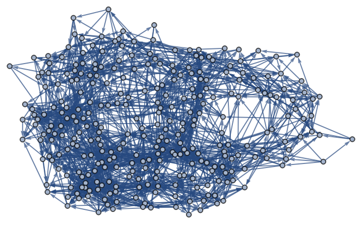
Fig 1
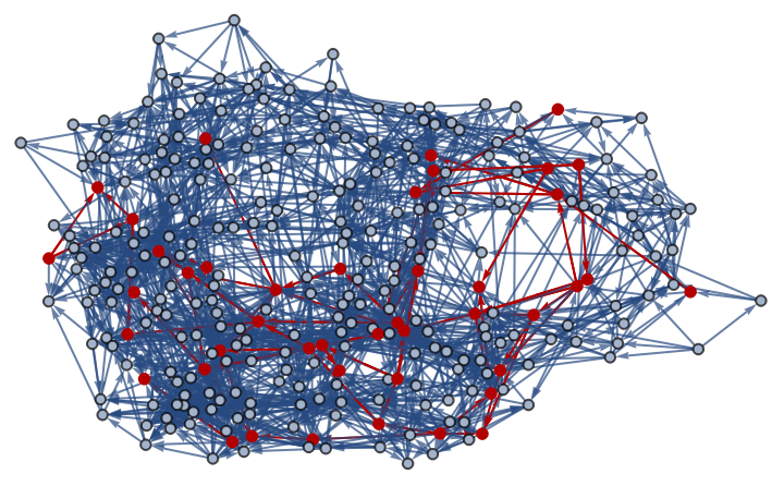
Fig 2
2. Bulk and Boundary Geometry:
2. Bulk and Boundary Geometry:
To analyze the bulk-boundary correspondence, we first need to define our bulk and boundary objects respectively. For an arbitrary boundary area A, we look for the corresponding bulk geodesic congruence.
◼
Boundary Construction:
We select two arbitrary points on the boundary and select all vertices within radial distance (r+discretization scale) from them. Here r is a user defined parameter and the discretization scale value is added to smoothen our discrete geometric setup. These spatially localized regions of the boundary of area A around the two points correspond to a discretized CFT setup.
◼
Bulk Construction:
We need to fix a spatial slice of bulk AdS. We use geodesic congruence to bound the bulk volume corresponding to the boundary area bounded by the CFT setup. In this project, we use the FindShortestPath function to draw a “straight line” between the two arbitrary boundary points selected above. We then select all points within a radial distance (r+discretization scale) from the line: this gives us an approximate geodesic cylinder with the two boundary “discs” marking its two endpoints. With this construction, we effectively force our Ryu-Takayanagi surface to encompass a specific “geodesic tube” on the causal graph corresponding to a boundary region of Area A. More rigorously, the geodesic congruence would be based on a family of geodesics(with all the same affine parameters.
γ)
3. Tensor Networks:
3. Tensor Networks:
With our construction, we force the bulk region to lie within the entropy cone of the boundary regions. Now we simply convert the boundary graphs obtained earlier into a tensor network. We implemented the following program that first converts any graph object into a corresponding directed tensor graph. This tensor graph is then converted into a quantum state using the Wolfram function . We can now obtain the density matrix and calculate the Von Neumann entropy.Note that we will obtain two tensor networks for the two “disc” objects on the boundary. We take a GraphUnion[] of the two and then calculate their aggregate entropy.
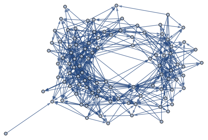
In this example, we work in a Kerr Newman geometry with mass and angular momentum as 1 and charge -1.
Here is the causal graph:
Here is the causal graph:
◼
GetTubes is the umbrella function that makes calls to both disk and geodesic tube generation:
◼
GenerateDisk generates the boundary subgraph and the resulting unionized boundary tensor graph:
Here we implement the boundary construction:
This is the tensor graph corresponding to the boundary:
◼
GenerateTubeGraph generates the bulk subgraph :
This is the bulk geometry for the given boundary:
4. Redundancy State Model:
4. Redundancy State Model:
Calculations
Calculations
◼
We calculated the mean entanglement entropy, mean hausdorff dimension, and mean Ricci Scalar Curvature for different geometries.
◼
Hausdorff Dimension of a causal graph
◼
Entanglement Entropy of a set of tensor graph:
◼
GetCorr gets the mean hausdorff dimension and mean entanglement entropy for an ensemble of bulk-boundary objects stored in geodesicList_:
◼
GetRicciScalar returns the mean Ricci Scalar Curvature value for an ensemble of bulk graphs:
Here is an example of a 7 dimensional Schwarzschild geometry:
◼
Causal Graph:
◼
Boundary Subgraph (highlighted in causal graph in Fig b):
Fig a Fig b
◼
geodesicList_ containing three pairs of disks(tensor networks) and geodesic tubes(causal subgraphs):
To verify the AdS/CFT correspondence, we expect to see a monotonic change in the bulk-boundary properties between different geometries. Here we have plotted three geometries in 3+1 dimensional spacetime: Kerr metric, AdS Schwarzschild metric, and Schwarzschild- with the following values of entropy, hausdorff dimension, and ricci scalar curvature:
◼
Entanglement Entropy vs Ricci Scalar Curvature:
◼
Entanglement Entropy vs Hausdorff Dimension:
Concluding remarks
Concluding remarks
With this project, we developed tools and concepts relevant to modelling AdS/CFT correspondence in the Wolfram framework. We designed a model for tensor networks to represent the underlying geometric relations and correlations and also built verifiable analogues for bulk and boundary properties, namely the Ricci Scalar Curvature and Hausdorff Dimensionality, and Entanglement Entropies, respectively.
We can see the expected monotonic behaviour in our plots but given the small sample size, no characteristic behavior could be definitely concluded from them.
We can see the expected monotonic behaviour in our plots but given the small sample size, no characteristic behavior could be definitely concluded from them.
Future Work
Future Work
◼
Extend calculations to other higher dimensional geometries to get more generalized results.
◼
Further develop optimization techniques and definitions to systematically demarcate bulk and boundary subgraphs.
◼
Develop a rigorous tensor network modeling tool for more complex structures like PIPS, MERA, etc.
◼
Investigate more concretely the tools and findings made to the AdS/CFT correspondence within the Wolfram models.
Keywords
Keywords
◼
AdS/CFT Correspondence
◼
Tensor Networks
References
References
[1] Cao, C., Carroll, S. M., & Michalakis, S. (2017). Space from Hilbert space: recovering geometry from bulk entanglement. Physical Review D, 95(2), 024031.
[2] Faulkner, Thomas, Monica Guica, Thomas Hartman, Robert C. Myers, and Mark Van Raamsdonk. “Gravitation from entanglement in holographic CFTs.” Journal of High Energy Physics 2014, no. 3 (2014): 1-41.
[3] Swingle, Brian. “Entanglement Renormalization and Holography.” Physical Review D, vol. 86, no. 6, Sept. 2012. Crossref, https://doi.org/10.1103/physrevd.86.065007.
[4] Pastawski, Fernando, Beni Yoshida, Daniel Harlow, and John Preskill. “Holographic quantum error-correcting codes: Toy models for the bulk/boundary correspondence.” Journal of High Energy Physics 2015, no. 6 (2015): 1-55.
CITE THIS NOTEBOOK
CITE THIS NOTEBOOK
Exploring the AdS/CFT correspondence in discrete spacetimes via tensor networks
by Srishti Nautiyal
Wolfram Community, STAFF PICKS, July 24, 2023
https://community.wolfram.com/groups/-/m/t/2975414
by Srishti Nautiyal
Wolfram Community, STAFF PICKS, July 24, 2023
https://community.wolfram.com/groups/-/m/t/2975414