Setup
Setup
This notebook needs exactly one companion file: the package DiachronicEmbeddings.wl, which holds all of the code and the small derived data it draws on (so no separate downloads, and not the 1.6 GB of raw HistWords embeddings). Put that file in the same folder as this notebook, then evaluate the cell below; every figure and table further down is then a single call to one of the package's functions.
GitHub: https://github.com/mthiel74/DiachronicWordEmbeddings
GitHub: https://github.com/mthiel74/DiachronicWordEmbeddings
Get[FileNameJoin[{NotebookDirectory[],"DiachronicEmbeddings.wl"}]]
deHero[]
1800s 1990s |
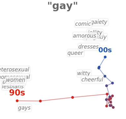
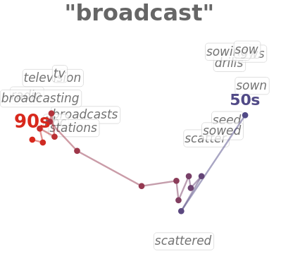
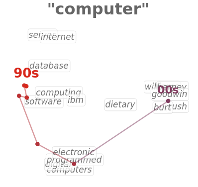
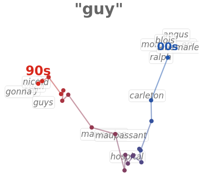
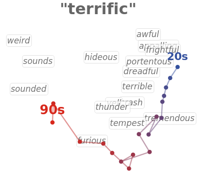
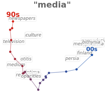
Figure. Six words, two centuries. Each panel projects one word's per-decade vector – blue in the 1800s, red in the 1990s – into a 2-D map of its own changing neighbourhood. §5 lets you explore any of the fourteen words interactively.
Word meanings move. Gay once meant carefree; broadcast meant to scatter seed by hand; a computer was a person who did arithmetic. This notebook makes that motion visible and measurable. Using the HistWords embeddings (word2vec / SGNS trained on the Google N-grams English corpus, one model per decade from the 1800s to the 1990s), we bring two centuries of independently-trained vector spaces into a single comparable frame with orthogonal Procrustes alignment, then trace individual words as trajectories through a 2-D projection of that shared space.
The drifting paths are the heart of the post (and §5 turns them into an interactive explorer). We then test, on the same aligned embeddings, the two statistical laws of semantic change of Hamilton, Leskovec & Jurafsky (2016): the law of conformity (frequent words drift more slowly) replicates cleanly, while the law of innovation (polysemous words drift faster) turns out to be a frequency confound in this corpus – a useful reminder to control before concluding. Everything is computed in the Wolfram Language; the code and data are in the companion repository.
1. The idea: words as moving points
1. The idea: words as moving points
A word embedding places every word at a point in a high-dimensional space so that words appearing in similar contexts land close together. Cosine similarity between two vectors then behaves like a similarity of meaning: in a modern embedding, king sits near queen and throne, far from pizza.
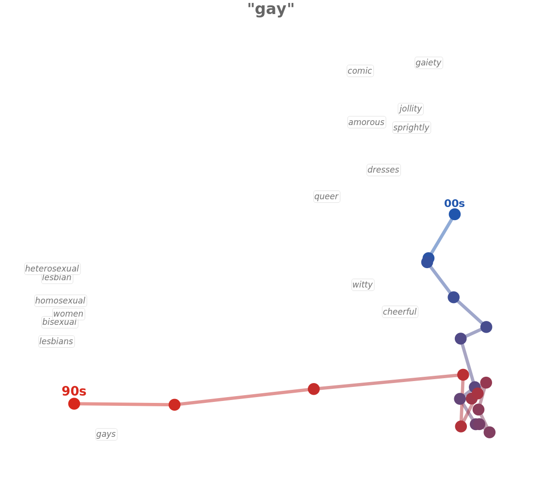
Now train one embedding on text from the 1850s and another on text from the 1990s. A word whose meaning has changed will sit in a different neighbourhood on the two maps. Gay keeps company with cheerful, merry, lively in the 1850s and with homosexual, lesbian, bisexual in the 1990s. If we can line the two maps up, that change becomes a displacement we can draw – and across twenty decades, a path.
Takeaway. Meaning change shows up as a word moving relative to the rest of the vocabulary. The whole project is about measuring and drawing that motion honestly.
2. The data: HistWords decade embeddings
2. The data: HistWords decade embeddings
We use the HistWords embeddings of Hamilton et al.: 300-dimensional skip-gram-with-negative-sampling (SGNS) vectors, trained separately for each decade on the Google N-grams eng-all corpus, from the 1800s through the 1990s – twenty decade-models, each with a 100,000-word vocabulary. The vectors are L2-normalized; a word absent from a decade is stored as a zero vector and skipped. The raw download is ~1.6 GB and is not committed; a thin Python shim converts the NumPy/pickle files to plain float32 binaries, and everything downstream is Wolfram Language.
Coverage varies by word. Of the fourteen we track, gay, awful, literally, nice, mouse and web appear in all twenty decades; queer from the 1830s, broadcast from the 1850s, and computer at 1900 (the human-“computer” sense) then continuously from the 1940s (the machine). Gaps are drawn as dashed segments. The full word list is deWords[].
3. Why the decades must be aligned
3. Why the decades must be aligned
Each decade's embedding is trained independently, so its coordinate axes are arbitrary: two decade-maps can be rotated and reflected relative to one another even when they agree perfectly about which words are near which. (A skip-gram objective is invariant under any orthogonal transformation of the space, so nothing pins down a shared orientation.) Before a word can be tracked through time, the decades must be rotated into a common frame.
We use orthogonal Procrustes alignment. Let A hold the vectors of the 5,000 highest-frequency words present in every decade, for one decade, and B the same words in the 1990s reference. We seek the orthogonal R minimising
argmin
R
2
AR-B
T
R
This has a closed form from a singular value decomposition: if U S V = AB, then R = U V. Because R is orthogonal it preserves every length and angle within a decade – it only reorients the space – so each decade's nearest neighbours are exactly as trained, while becoming comparable across decades. (Nearest-neighbour queries in §6 are therefore run in each decade's own native space; alignment is needed only to compare frames.)
deAlignmentPlot[]
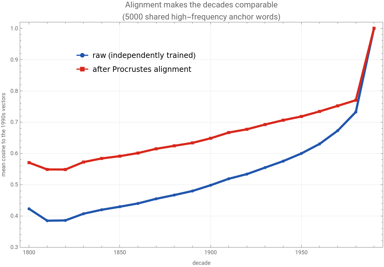
Figure. Mean cosine of the 5,000 shared anchor words to their 1990s vectors, before (blue) and after (red) Procrustes alignment. Alignment lifts the curve at every decade; both necessarily reach 1.0 at the 1990s reference.
How far from comparable are the raw spaces? The rotation that best aligns the 1800s onto the 1990s is large: R − I = 21.20. For calibration, two unrelated 300-D spaces are related by a random rotation with R − I ≈ 24.50, identical spaces give 0, and a perfect mirror-flip gives the maximum 34.60. So the 1800s axes begin almost as unrelated to the 1990s as random – alignment is essential, not cosmetic – and the required rotation then shrinks smoothly toward the present.
Aligning lifts the mean anchor-word cosine to the 1990s at every decade (1800s: 0.42 0.57; 1900s: 0.50 0.65). That the raw (blue) curve already rises, rather than sitting near zero, is itself informative: HistWords initialises each decade's training from the previous one, so adjacent decades inherit a partial common orientation – but that shared frame erodes over a century, which is exactly why distant decades must be re-aligned. The numbers above come from deAlignmentFacts[].
Takeaway. Independently trained spaces are not comparable as shipped. One orthogonal rotation per decade, fitted on stable high-frequency words, makes them comparable while leaving each decade's internal geometry untouched.
4. How to read a trajectory
4. How to read a trajectory
For one word we collect its aligned vector in every decade it occurs, gather the nearest neighbours that anchor each era of its meaning, and project that whole local neighbourhood to two dimensions with PCA. The word's path then threads between an early-meaning cluster and a late-meaning cluster; colour runs from blue (1800s) to red (1990s). One call draws any word:
deTrajectoryPlot["gay"]
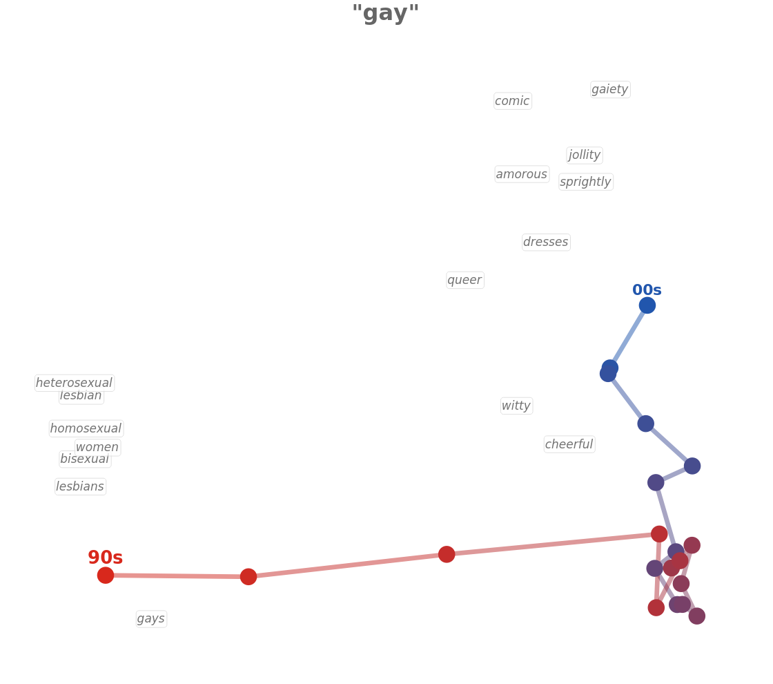
Figure. gay: the path lingers among merry, cheerful, joyous, lively, gaiety through the blue and purple decades, then swings sharply red-ward to homosexual, lesbian, gays, bisexual by the 1990s – a two-century meaning change rendered as a single sweep.
What the projection does and does not say. The 2-D layout is a per-word PCA of that word's own cloud, chosen to spread its motion across the page; absolute positions and the axes themselves carry no global meaning, and 2-D distances are an approximation of the true 300-D ones. The trustworthy signal is which neighbours sit at each end of the path and how far the word travels between them – both of which come straight from the high-dimensional cosine geometry, not the projection.
Takeaway. Read a trajectory by its endpoints and their neighbours, not by the exact shape of the curve. The neighbours are the evidence; the curve is just their geometry.
5. Explore all fourteen words
5. Explore all fourteen words
Rather than print fourteen separate plots, the same construction is wired into one interactive Manipulate. Pick a word, scrub the time slider to reveal the path decade by decade, and toggle the neighbour labels. (Opened in the Wolfram notebook the controls are live immediately – no need to re-evaluate; a static export such as the PDF shows a single frame, gay with its full path.)
deExplorer[]


A few worth visiting: broadcast (agricultural sow / seed / scatter radio / television / bbc); computer (a V from human surnames through electronic / circuits to software / internet); mouse (keeps rat / cat but grows a second cursor / click / keyboard cluster); web (spider www / browser / server); terrific and awful (the two halves of a terror-to-praise swap); and guy (the Guy Fawkes effigy fellow / chap / dude).
Not every famous case shows up cleanly, and the explorer is honest about that. literally is the textbook example of a meaning change – the modern hyperbolic intensifier – yet in this corpus its neighbours stay anchored to literal, figuratively, metaphorically across all twenty decades, with only a faint late drift toward thousands, hundreds, utterly. The intensifier sense is mostly a spoken-register phenomenon that the edited-book Google N-grams corpus barely records, so the embedding has little to latch onto. A real reminder that absence of measured drift is not absence of change – only absence of evidence in this corpus.
6. Nearest-neighbour drift tables
6. Nearest-neighbour drift tables
The trajectories are the geometry of a simpler fact: the list of a word's nearest neighbours turns over from decade to decade. Neighbours are computed by cosine similarity in each decade's own native space. Sampled every fifty years:
Figure. Top-5 cosine nearest neighbours by decade. Any subset of deWords[] can be passed to deNeighborTable.
Takeaway. Trajectories can be cross-checked against plain word lists. When the neighbours of broadcast go from sow, scatter to radio, television, the drawn path is just reporting that shift.
7. Two statistical laws of semantic change
7. Two statistical laws of semantic change
Hamilton, Leskovec & Jurafsky (2016) propose two regularities of semantic change. Both can be tested directly on the aligned embeddings, measured over the 11332 dictionary content words present in every decade (function words and archaic/foreign tokens removed via a stoplist and WordData membership). A word's rate of change is the mean cosine distance between its aligned vectors in consecutive decades; its frequency is proxied by its mean rank, and its polysemy by its number of WordNet senses. Re-deriving the laws independently is also a good way to watch a confound masquerade as a result. (Statistics: deLawFacts[].)
The law of conformity – holds
The law of conformity – holds
More frequent words change more slowly. Change-rate falls steeply with frequency (Spearman ρ = -0.94, slope -0.12 in log-rate). Why: a high-frequency word is seen in a huge range of contexts, so its vector is an average over many uses and is statistically well-anchored. Part of the strength is also methodological – rare words are estimated from little data, so their vectors are noisier and look like they move more – which is itself worth stating plainly.
Figure. Rate of semantic change vs. frequency (−log mean rank). Red markers are decile means.
The law of innovation – a cautionary tale
The law of innovation – a cautionary tale
The published law says more polysemous words change faster. In this corpus the raw correlation comes out the wrong way: change-rate vs. polysemy has Spearman ρ = -0.31 – negative. The culprit is a confound: polysemous words tend to be frequent (ρ = 0.34), and frequency strongly suppresses change. In the raw comparison the frequency effect simply dominates – a textbook Simpson's paradox.
Controlling for frequency (partial Spearman correlation, holding frequency rank fixed) the spurious negative trend vanishes – but it does not turn convincingly positive either: partial ρ = 0.01, essentially zero. So in the Google-N-grams eng-all corpus, with WordNet sense counts as the polysemy measure, the law of innovation does not replicate. That is a more honest – and more useful – result than forcing the sign: the law may need a different corpus, a better polysemy measure, or the original authors' frequency-and-polysemy-matched controls to surface.
Figure. The raw polysemy trend (blue) slopes the "wrong" way only because polysemous words are frequent; the frequency-controlled residual (red) is flat. Raw Spearman -0.31, partial 0.01.
Takeaway. Conformity replicates cleanly; innovation does not survive a frequency control here. A large raw correlation is easy to get and easy to misread – always ask what else moves with your variable before naming an effect.
8. The most-drifted words – and a caveat
8. The most-drifted words – and a caveat
Ranking every stable content word by how far it moved between its 1800s and 1990s aligned vectors surfaces two phenomena at once. Some entries are genuine meaning change (advert verb noun, peer noble equal, media, broadcast); others are lexical obsolescence or register shift, where an archaic word (twelvemonth, fourthly, civilities) simply stopped occurring in the same kinds of text. A large embedding displacement means “the contexts changed” – which is necessary, but not sufficient, for “the meaning changed”. Distinguishing the two is where embeddings end and lexicography begins.
Figure. The 25 most-drifted stable content words, 1800s–1990s. The full ranking is in data/drift_ranking.json.
Takeaway. Embeddings are a powerful detector of that something changed about a word's usage; deciding what changed still needs the neighbour lists, the trajectories, and human judgement.
9. Methods and reproduction
9. Methods and reproduction
Every output above is a single call to a function in the companion package DiachronicEmbeddings.wl attached alongside this notebook. That one file is self-contained: it carries both the code and the small derived data products it draws on, so the notebook runs from just the two uploaded files. (In the source repository the same code lives un-bundled as wolfram/DiachronicEmbeddings.wl with the data split out under data/; community/bundle_package.wls is what folds the two together into the uploadable file.) To regenerate the data products from scratch (the science is pure Wolfram Language; the only Python is a NumPy/pickle format shim):
◼
wolframscript -file wolfram/fetch_data.wls – download + unzip the HistWords eng-all SGNS embeddings
◼
python3 src/convert_histwords.py – .npy/.pkl float32 binaries + vocab (anchors, targets, pools)
◼
wolframscript -file wolfram/trajectories.wls – Procrustes alignment, projection trajectories.json + neighbors.json
◼
wolframscript -file wolfram/laws_and_drift.wls – drift leaderboard + the two laws laws.json, laws_points.json, drift_ranking.json
◼
wolframscript -file wolfram/alignment.wls – the alignment diagnostic alignment.json
Repository: github.com/mthiel74/DiachronicWordEmbeddings.
10. Data, licensing, and acknowledgements
10. Data, licensing, and acknowledgements
This notebook builds entirely on freely-reusable data, and redistributes only small derived products of it – 2-D trajectory coordinates, nearest-neighbour word lists, and the alignment and law statistics.
◼
HistWords embeddings. The per-decade SGNS vectors are from the HistWords project (Hamilton, Leskovec & Jurafsky), released into the public domain under the Open Data Commons Public Domain Dedication and License (PDDL) v1.0. Redistribution of the embeddings and of products derived from them is therefore unrestricted; as the project requests, the source paper is cited below.
◼
Google Books N-grams. Those embeddings were trained on the Google Books Ngram eng-all corpus, released by Google under the Creative Commons Attribution 3.0 (CC BY 3.0) licence (Google Books Ngram Viewer, books.google.com/ngrams).
◼
WordNet. The polysemy measure in §7 uses WordNet sense counts via WordData. WordNet is © Princeton University, made available under a permissive free licence (attribution).
◼
This notebook's code. The package DiachronicEmbeddings.wl and the rest of the companion repository are released into the public domain (The Unlicense) – reuse, modify, or sell freely, with no conditions and no attribution required. No HistWords source code is redistributed here – only the public-domain data products – so the HistWords tools' Apache-2.0 licence does not apply.
In short: the data carries no copyright restriction, the corpus and WordNet ask only for attribution (given here), and the code is MIT. The post is free to read, run, and build on.
11. References
11. References
W. L. Hamilton, J. Leskovec, D. Jurafsky (2016). Diachronic Word Embeddings Reveal Statistical Laws of Semantic Change. ACL 2016. arXiv:1605.09096.
P. H. Schönemann (1966). A generalized solution of the orthogonal Procrustes problem. Psychometrika 31(1). (The SVD alignment used in §3.)
T. Mikolov et al. (2013). Distributed Representations of Words and Phrases and their Compositionality. NeurIPS 2013. (word2vec / SGNS.)
V. Kulkarni et al. (2015). Statistically Significant Detection of Linguistic Change. WWW 2015.
J.-B. Michel et al. (2011). Quantitative Analysis of Culture Using Millions of Digitized Books. Science 331. (The Google N-grams corpus.)
CITE THIS NOTEBOOK
CITE THIS NOTEBOOK
Diachronic word embeddings: 200 years of semantic drift, traced through a embedding space
by Marco Thiel
Wolfram Community, STAFF PICKS, June 3, 2026
https://community.wolfram.com/groups/-/m/t/3726644
by Marco Thiel
Wolfram Community, STAFF PICKS, June 3, 2026
https://community.wolfram.com/groups/-/m/t/3726644