ABSTRACT (original article): We study the problem of minimising the connection time between non-equilibrium steady states of the Brownian Gyrator. This is a paradigmatic model in non-equilibrium statistical mechanics, an overdamped Brownian particle trapped in a two-dimensional elliptical potential, with the two degrees of freedom coupled to two, in principle different, thermal baths with temperatures and , respectively. Application of Pontryagin’s Maximum Principle reveals that shortest protocols belong to the boundaries of the control set defined by the limiting values of the parameters characterising the elliptical potential. We identify two classes of optimal minimum time protocols, i.e. brachistochrones: (i) regular bang-bang protocols, for which alternatively take their minimum and maximum values allowed, and (ii) infinitely degenerate singular protocols. We thoroughly investigate the minimum connection time over the brachistochrones in the limit of having infinite capacity for compression. A plethora of striking phenomena emerge: sets of states attained at null connection times, discontinuities in the connection time along adjacent target states, and the fact that, starting from a state in which the oscillators are coupled, uncoupled states are impossible to reach in a finite time. CITATION (original article): A. Patrón, C. A. Plata and A. Prados (2024), Minimum time connection between non-equilibrium steady states: the Brownian gyrator, arXiv:2407.21110. https://doi.org/10.48550/arXiv.2407.21110
(x,y)
T
x
T
y
(k,u)
(k,u)
In this notebook we provide the numerical computations employed for the paper “Minimum time connection between non-equilibrium steady states: the Brownian Gyrator”, A. Patrón, C. A. Plata and A. Prados (arXiv:2407.21110).
ResourceFunction["MaTeXInstall"][]<<MaTeX`SetOptions[MaTeX,"Preamble"->{"\\usepackage{color}"}];
Reachable states for optimal bang-bang protocols (Figures 4, 5 and 6)
Reachable states for optimal bang-bang protocols (Figures 4, 5 and 6)
Here, given a fixed initial state (, ), we determine the reachable regions in the (, )-space by means of optimal bang-bang protocols (one, two and three bangs specifically), which switch between the three different vertices of the triangle-shaped control set for the parameters (): O (() = (0,0)), P (() = (, )) and N (() = (, )), with ∞. In the following, A -> Vertex O. B -> Vertex P, C -> Vertex N.
k
i
u
i
k
f
u
f
k,u
k,u
k,u
k
max
k
max
k,u
k
max
-
k
max
k
max
Initial parameters:
uini=0.5;kini=1.0;km=4;
Limiting curve for the NOP (CAB) bang-bang protocol
Limiting curve for the NOP (CAB) bang-bang protocol
This protocol is numerically unstable in comparison with the rest of the bang-bang ones, such that we obtain its corresponding limiting region using a discretisation method in the (, )-space.
k
f
u
f
tfCAB[x_,y_]:=Piecewise[{{Min[tf/.NSolve[{1/(x+y)(1/(kini+uini)+2*tf)*u^2,1/(x-y)w^2/(kini-uini)+2*(tf),1/x(w/kini+2*tf)*u,u>0,u<1,w>0,w<1},{tf,w,u}][[2]],tf/.NSolve[{1/(x+y)(1/(kini+uini)+2*tf)*u^2,1/(x-y)w^2/(kini-uini)+2*(tf),1/x(w/kini+2*tf)*u,u>0,u<1,w>0,w<1},{tf,w,u}][[1]]],Length[NSolve[{1/(x+y)(1/(kini+uini)+2*tf)*u^2,1/(x-y)w^2/(kini-uini)+2*(tf),1/x(w/kini+2*tf)*u,u>0,u<1,w>0,w<1},{tf,w,u}]]>1.5},{tf/.NSolve[{1/(x+y)(1/(kini+uini)+2*tf)*u^2,1/(x-y)w^2/(kini-uini)+2*(tf),1/x(w/kini+2*tf)*u,u>0,u<1,w>0,w<1},{tf,w,u}][[1]],1.5>Length[NSolve[{1/(x+y)(1/(kini+uini)+2*tf)*u^2,1/(x-y)w^2/(kini-uini)+2*(tf),1/x(w/kini+2*tf)*u,u>0,u<1,w>0,w<1},{tf,w,u}]]>0.5},{{},Length[NSolve[{1/(x+y)(1/(kini+uini)+2*tf)*u^2,1/(x-y)w^2/(kini-uini)+2*(tf),1/x(w/kini+2*tf)*u,u>0,u<1,w>0,w<1},{tf,w,u}]]<0.5}}]
vec={};ϵk=0.02;ϵu=0.0025;For[i=1,i<201,i++,k=ϵk*i;Nsteps=uini*k/ϵu;uvar=Select[Table[{ϵu*j,tfCAB[k,ϵu*j]},{j,0,Nsteps}],UnsameQ[#[[2]],{}]&][[1]][[1]];AppendTo[vec,{k,uvar}];Print[k]]
Export["file path for 'tfNOP.dat'",vec]
The above allows to obtain the ‘tfNOP.dat’ file, which is employed directly in the plots from the following figures.
Evolution equations for the two - bang protocols
Evolution equations for the two - bang protocols
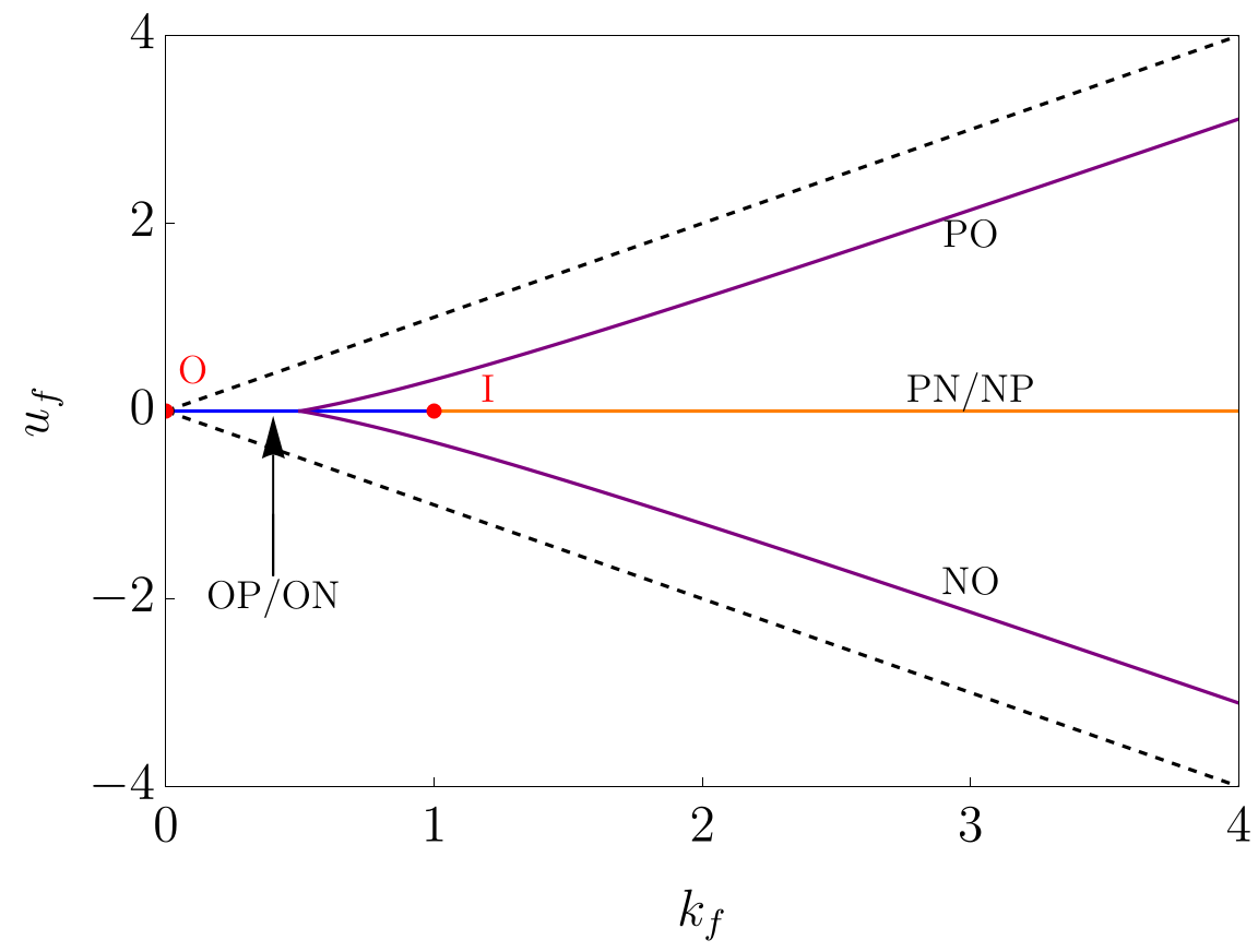
Figure 4 : Map of two - bang protocols
Figure 4 : Map of two - bang protocols
u0fun[k_,σ_]:=σ*k*(2*k-1)/(2*k+1);ShowPlot[{0},{k,0,1},PlotStyleBlue],Plot[{0},{k,1,kmax},PlotStyleOrange],Plot[{u0fun[k,1],u0fun[k,-1]},{k,0.5,kmax},PlotStylePurple],Plot[{k},{k,0,kmax},PlotStyle{Black,Dashed}],Plot[{-k},{k,0,kmax},PlotStyle{Black,Dashed}],Frame->True,FrameStyleDirective[Black,28,FontFamily"Times New Roman"],
ShowPlot[{ufunOP[k]},{k,0,kmax},PlotStyleBlue],Plot[{ufunPN[k]},{k,1,kmax},PlotStyleOrange],Plot[{-ufunPN[k]},{k,3,kmax},PlotStyleOrange],Plot[{ufunON[k]},{k,0,kmax},PlotStyleBlue],Plot[{ufunPO1[k],ufunPO2[k],ufunPO3[k]},{k,0,kmax},PlotStylePurple],Plot[{ufunNO1[k],ufunNO2[k],ufunNO3[k]},{k,0,kmax},PlotStylePurple],Plot[{k},{k,0,kmax},PlotStyle{Black,Dashed}],Plot[{-k},{k,0,kmax},PlotStyle{Black,Dashed}],
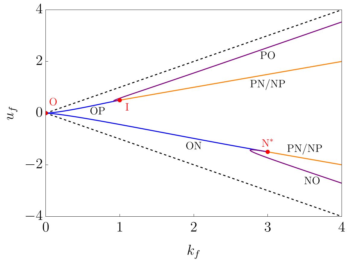
Figures 5 and 6 : Map of three - bang protocols
Figures 5 and 6 : Map of three - bang protocols
Export["file path for 'two_bang_map.pdf'",p1]
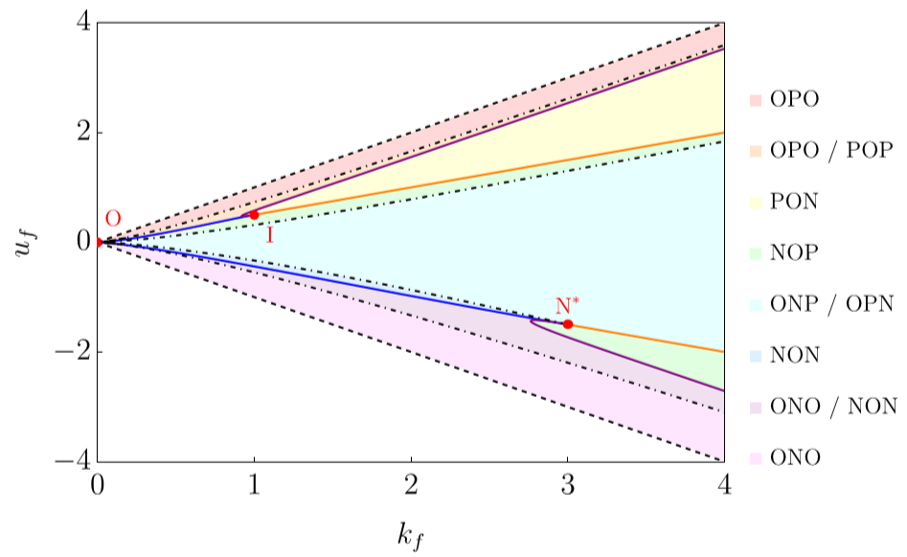
p2=ShowRegionPlot[2*tf1[x,y,kini,0]>(x+y)/x^2&&y<x&&y>0,{x,0,km},{y,-km,km},PlotStyle->LightRed,BoundaryStyle->None,PlotLegends->MaTeX[{"\\text{OPO}"},Magnification->1.5],PlotPoints->100],RegionPlot[2*tf1[x,y,kini,0]<(x+y)/x^2&&y>x*(2*x-1)/(2*x+1)&&y<x&&y>0,{x,0,km},{y,-km,km},PlotStyle->LightOrange,BoundaryStyle->None,PlotLegends->MaTeX[{"\\text{OPO / POP}"},Magnification->1.5],PlotPoints->200],RegionPlot[y<x*(2*x-1)/(2*x+1)&&y<x&&y>0,{x,0,km},{y,-km,km},PlotStyle->LightYellow,BoundaryStyle->None,PlotLegends->MaTeX[{"\\text{PON}"},Magnification->1.5],PlotPoints->100],RegionPlot[y>-x*(2*x-1)/(2*x+1)&&y<x&&y<0,{x,0,km},{y,-km,km},PlotStyle->LightGreen,BoundaryStyle->None,PlotLegends->MaTeX[{"\\text{NOP}"},Magnification->1.5],PlotPoints->100],RegionPlot[2*tf2[x,y,kini,0]<(x-y)/x^2&&y<-x*(2*x-1)/(2*x+1)&&y<x&&y<0&&y>-x,{x,0,km},{y,-km,km},PlotStyle->LightPurple,BoundaryStyle->None,PlotLegends->MaTeX[{"\\text{ONO / NON}"},Magnification->1.5],PlotPoints->200],RegionPlot[2*tf2[x,y,kini,0]>(x-y)/x^2&&y>-x&&y<0,{x,0,km},{y,-km,km},PlotStyle->LightMagenta,BoundaryStyle->None,PlotLegends->MaTeX[{"\\text{ONO}"},Magnification->1.5],PlotPoints->100],ContourPlot[2*tf2[x,y,kini,0]==(x-y)/x^2,{x,0,km},{y,-km,0},ContourStyle->{Black,DotDashed}],ContourPlot[2*tf1[x,y,kini,0]==(x+y)/x^2,{x,0,km},{y,0,km},ContourStyle->{Black,DotDashed}],Plot[{0},{k,0,1},PlotStyleBlue],Plot[{0},{k,1,km},PlotStyleOrange],Plot[{u0fun[k,1],u0fun[k,-1]},{k,0.5,km},PlotStylePurple],Plot[{k},{k,0,km},PlotStyle{Black,Dashed}],Plot[{-k},{k,0,km},PlotStyle{Black,Dashed}],
Initial parameters:
Figure 7 left: density plot
Figure 7 left: density plot
Initial parameters:
Figure 7 right: density plot
Figure 7 right: density plot
Initial parameters:
Figure 7, left panels
Figure 7, left panels
Initial parameters:
Figure 7, right panels
Figure 7, right panels
CITE THIS NOTEBOOK
CITE THIS NOTEBOOK
Minimum time connection between non-equilibrium steady states: the Brownian gyrator
by A. Patrón, C. A. Plata, A. Prados
Wolfram Community, STAFF PICKS, September 24, 2024
https://community.wolfram.com/groups/-/m/t/3282502
by A. Patrón, C. A. Plata, A. Prados
Wolfram Community, STAFF PICKS, September 24, 2024
https://community.wolfram.com/groups/-/m/t/3282502