Residue Curves for a Reactive Ternary System
Authors: Housam Binous and Ahmed Bellagi
Residue Curves for a Reactive Ternary System
Authors: Housam Binous and Ahmed Bellagi
Authors: Housam Binous and Ahmed Bellagi
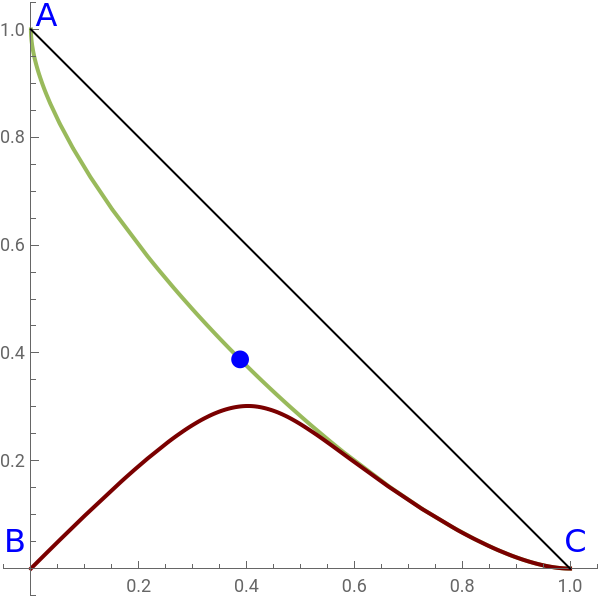
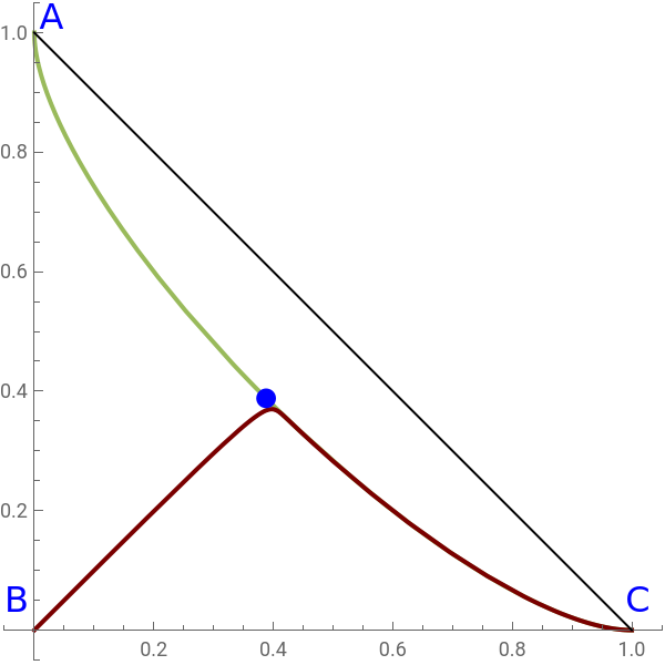
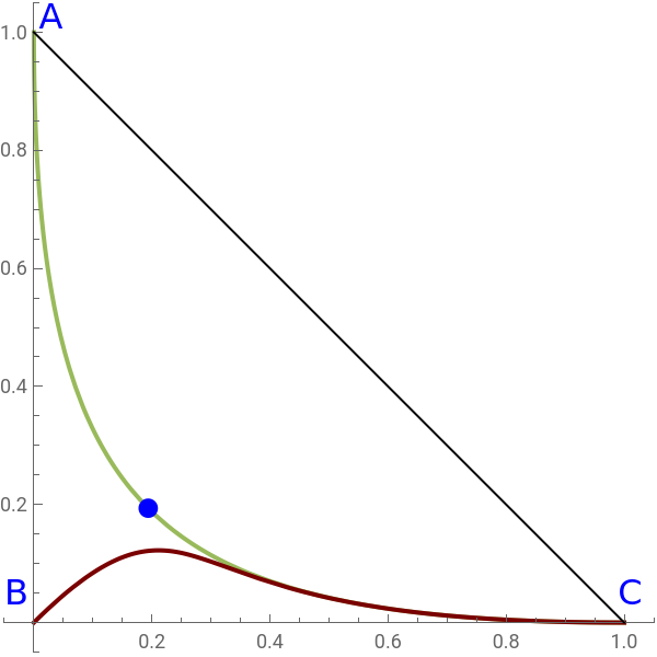
Consider an ideal ternary mixture subject to an equilibrium-limited chemical reaction . The relative volatilities are taken as =5 and =3. Pure is fed to the still. We plots the residue curve (red) for this ternary reactive mixture as well as the equilibrium curve (green). It is clear that as the value of the Damköhler number, , becomes large, the residue curve approaches the equilibrium curve more rapidly. After some time, both curves will overlap for high . Only component will be left in the still after a long enough time. You can vary the Damköhler number as well as the equilibrium constant and see the effect on both the residue curve and the equilibrium curve. Ref. 1 by Doherty and Malone contains detailed information both for residue curve of nonreactive and reactive mixtures.
Let us explain the observed behavior:
Initially only species is fed to the still. Reaction produces some A and C. However, the most volatile component A will leave the still, which will displaces the equilibrium toward more depletion of B, the result will be all B is consumed and only C (the heaviest species) will remain in the still. This is further confirmed by the fact that the residue curve shown in red end up at the corner of the ternary diagram corresponding to pure C.
References:
[1] M.F.Doherty and M.F.Malone, Conceptual Design of Distillation Systems, Boston : McGraw - Hill, 2001.
2B⇌A+C
α
AC
α
BC
B
Da
Da
C
Let us explain the observed behavior:
Initially only species
B
2B⇌A+C
References:
[1] M.F.Doherty and M.F.Malone, Conceptual Design of Distillation Systems, Boston : McGraw - Hill, 2001.
In[]:=
rate[t_]:=x2[t]^2-x1[t]x3[t]/Keq;(*rateofreactionexpressionfor2B⇌A+C*)
In[]:=
α13=5;α23=3;(*assumeidealmixturewithconstantrelativevolatilities*)
In[]:=
(*VLErelations*)y1[t_]:=α13x1[t]/(α13x1[t]+α23x2[t]+x3[t]);y2[t_]:=α23x2[t]/(α13x1[t]+α23x2[t]+x3[t]);y3[t_]:=x3[t]/(α13x1[t]+α23x2[t]+x3[t]);
In[]:=
x3[t_]:=1-x1[t]-x2[t];(*summationrules*)
CASE 1
In[]:=
Da=5;Keq=3;
In[]:=
x2f=x2/.FindRoot[1-2x2+-4Keq0,{x2,0.25}](*thisvaluehelpidentifythelocusofthebluedot*)
2
x2
2
x2
Out[]=
0.224009
In[]:=
sol=NDSolve[Flatten[{D[x1[t],{t,1}]x1[t]-y1[t]+Da(1)rate[t],D[x2[t],{t,1}]x2[t]-y2[t]+Da(-2)rate[t],x1[0]0.,x2[0]1.0}],{x1[t],x2[t]},{t,0,10},Method->"StiffnessSwitching"];(*residuecurvecomputation*)
In[]:=
rc=Show[ParametricPlot[{First[x3[t]/.sol],First[x1[t]/.sol]},{t,0,10},PlotStyle{Thick,RGBColor[0.48,0,0]},ImageSize300{1,1},PlotRange{{-0.05,1.05},{-0.05,1.05}},Epilog{Black,Line[{{0,1},{1,0}}]}]];(*residuecurveplotting*)
eq=ParametricPlot1-x2+1-x2-1-x2-1-x2+
1
2
1-2x2+-4Keq
,2
x2
2
x2
1
2
1-2x2+-4Keq
,2
x2
2
x2
1
2
1-2x2+-4Keq
,2
x2
2
x2
1
2
1-2x2+-4Keq
,{x2,0,1},PlotStyle{{Thick,RGBColor[.6,.73,.36]},{Thick,RGBColor[.6,.73,.36]}},ImageSize300{1,1},PlotRange{{-0.05,1.05},{-0.05,1.05}},Epilog{Black,Line[{{0,1},{1,0}}]};(*equilibriumcurve*)2
x2
2
x2
In[]:=
Showeq,rc,GraphicsBlue,Style[Text["B",{-0.0295,0.05}],16],Style[Text["A",{0.029,1.025}],16],Style[Text["C",{1.01,0.05}],16],Blue,PointSize[0.03],Point1-x2f+1-x2f-
1
2
1-2x2f+-4Keq
,2
x2f
2
x2f
1
2
1-2x2f+-4Keq
2
x2f
2
x2f
Out[]=
CASE 2
In[]:=
Da=50;Keq=3;
In[]:=
x2f=x2/.FindRoot[1-2x2+-4Keq0,{x2,0.25}](*thisvaluehelpidentifythelocusofthebluedot*)
2
x2
2
x2
Out[]=
0.224009
In[]:=
sol=NDSolve[Flatten[{D[x1[t],{t,1}]x1[t]-y1[t]+Da(1)rate[t],D[x2[t],{t,1}]x2[t]-y2[t]+Da(-2)rate[t],x1[0]0.,x2[0]1.0}],{x1[t],x2[t]},{t,0,10},Method->"StiffnessSwitching"];(*residuecurvecomputation*)
In[]:=
rc=Show[ParametricPlot[{First[x3[t]/.sol],First[x1[t]/.sol]},{t,0,10},PlotStyle{Thick,RGBColor[0.48,0,0]},ImageSize300{1,1},PlotRange{{-0.05,1.05},{-0.05,1.05}},Epilog{Black,Line[{{0,1},{1,0}}]}]];(*residuecurveplotting*)
eq=ParametricPlot1-x2+1-x2-1-x2-1-x2+
1
2
1-2x2+-4Keq
,2
x2
2
x2
1
2
1-2x2+-4Keq
,2
x2
2
x2
1
2
1-2x2+-4Keq
,2
x2
2
x2
1
2
1-2x2+-4Keq
,{x2,0,1},PlotStyle{{Thick,RGBColor[.6,.73,.36]},{Thick,RGBColor[.6,.73,.36]}},ImageSize300{1,1},PlotRange{{-0.05,1.05},{-0.05,1.05}},PlotPoints->100,Epilog{Black,Line[{{0,1},{1,0}}]};(*equilibriumcurve*)2
x2
2
x2
In[]:=
Showeq,rc,GraphicsBlue,Style[Text["B",{-0.0295,0.05}],16],Style[Text["A",{0.029,1.025}],16],Style[Text["C",{1.01,0.05}],16],Blue,PointSize[0.03],Point1-x2f-1-x2f+
1
2
1-2x2f+-4Keq
,2
x2f
2
x2f
1
2
1-2x2f+-4Keq
2
x2f
2
x2f
Out[]=
CASE 3
In[]:=
Da=0.5;Keq=0.1;
In[]:=
x2f=x2/.FindRoot[1-2x2+-4Keq0,{x2,0.25}](*thisvaluehelpidentifythelocusofthebluedot*)
2
x2
2
x2
Out[]=
0.612574
In[]:=
sol=NDSolve[Flatten[{D[x1[t],{t,1}]x1[t]-y1[t]+Da(1)rate[t],D[x2[t],{t,1}]x2[t]-y2[t]+Da(-2)rate[t],x1[0]0.,x2[0]1.0}],{x1[t],x2[t]},{t,0,10},Method->"StiffnessSwitching"];(*residuecurvecomputation*)
In[]:=
rc=Show[ParametricPlot[{First[x3[t]/.sol],First[x1[t]/.sol]},{t,0,10},PlotStyle{Thick,RGBColor[0.48,0,0]},ImageSize300{1,1},PlotRange{{-0.05,1.05},{-0.05,1.05}},Epilog{Black,Line[{{0,1},{1,0}}]}]];(*residuecurveplotting*)
eq=ParametricPlot1-x2+1-x2-1-x2-1-x2+
1
2
1-2x2+-4Keq
,2
x2
2
x2
1
2
1-2x2+-4Keq
,2
x2
2
x2
1
2
1-2x2+-4Keq
,2
x2
2
x2
1
2
1-2x2+-4Keq
,{x2,0,1},PlotStyle{{Thick,RGBColor[.6,.73,.36]},{Thick,RGBColor[.6,.73,.36]}},ImageSize300{1,1},PlotRange{{-0.05,1.05},{-0.05,1.05}},Epilog{Black,Line[{{0,1},{1,0}}]};(*equilibriumcurve*)2
x2
2
x2
In[]:=
Showeq,rc,GraphicsBlue,Style[Text["B",{-0.0295,0.05}],16],Style[Text["A",{0.029,1.025}],16],Style[Text["C",{1.01,0.05}],16],Blue,PointSize[0.03],Point1-x2f+1-x2f-
1
2
1-2x2f+-4Keq
,2
x2f
2
x2f
1
2
1-2x2f+-4Keq
2
x2f
2
x2f
Out[]=
CASE 4
In[]:=
Da=5;Keq=0.1;
In[]:=
x2f=x2/.FindRoot[1-2x2+-4Keq0,{x2,0.25}](*thisvaluehelpidentifythelocusofthebluedot*)
2
x2
2
x2