Limitations of numerical methods as employed in spreadsheets
Limitations of numerical methods as employed in spreadsheets
Often, we use a naïve definition of a vector as an ordered (or indexed) finite sequence of scalars; it is usually represented in parenthesis as an n-tuple , , … , ), an element of Cartesian product = 𝔽 × 𝔽 × ⋯ × 𝔽 of n copies of the field of scalars 𝔽. Later, we will extend this definition to include abstract objects; however, for us at this moment, it is sufficient to work with n-tuples. Recall that for scalars we use either rational numbers ℚ or real numbers ℝ or complex numbers ℂ.
Usually, an n-tuple, , … , ), written in parenthesis and a row vector , , … , ], written in brackets, look as the same object to human eyes. One of the pedagogical virtues of any software package is its requirement to pay close attention to the types of objects used in specific contexts. In particular, the computer algebra system Mathematica treats these two versions of a vector differently because
(
x
1
x
2
x
n
n
𝔽
Usually, an n-tuple
(
x
1
x
2
x
n
[
x
1
x
2
x
n
{,,...,
x
1
x
2
x
n
n
but
{,,...,
x
1
x
2
x
n
mxn
where x [bold] is a matrix and is read “m by n” indicating dimensions of a 2 x 2 (or rows by columns) matrix, not m multiplied by n. This denotes the space of m × n matrices with coefficients from field 𝔽. Mathematica considers single bracket notation as a matrix with one column and a double bracket notation as a matrix with one row.
mxn
𝔽
In[]:=
x={1,2};(*onecolumnmatrix*)y={{1,2}};(*onerowmatrix*)TrueQ[x==y]
Out[]=
False
In[]:=
MatrixForm[x]
Out[]//MatrixForm=
1 |
2 |
In[]:=
MatrixForm[y]
Out[]//MatrixForm=
(
)
1 | 2 |
Note that dot product of these objects is non-commutative. That is, the order matters
In[]:=
x.y

Out[]=
{1,2}.{{1,2}}
In[]:=
y.x
Out[]=
{5}
A hint at the reason this distinction is important is found in the word “Tensors” in the error message above. This refers to the physics notation that ignores columns and rows and considers the matter one of “levels.” Note that Level 1 (Part 1 in the Wolfram language) is a scalar
In[]:=
x[[1]]%//MatrixForm
Out[]=
1
Out[]//MatrixForm=
1
For y, the first element is a list...
In[]:=
y[[1]]
Out[]=
{1,2}
...and to access an element lower - which is inside that list - one must go down another level and is a scalar.
In[]:=
y[[1,2]]
Out[]=
2
The matrix as a special case
The matrix as a special case
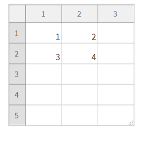
Two element, single column or single row, matrices are not very interesting. Note what happens when we have a 2 x 2 matrix
In[]:=
z={{1,2},{3,4}};MatrixForm[%]
Out[]//MatrixForm=
1 | 2 |
3 | 4 |
There are two components, each a list, in Level 1 of z. Each of these is a row of the matrix z
In[]:=
z[[1]]
Out[]=
{1,2}
In[]:=
z[[2]]
Out[]=
{3,4}
We can ask for Level 2 details by asking Part for the second element in second component (element) of Level 1, a scalar in this case.
In[]:=
z[[2,2]]
Out[]=
4
All of this accommodates the fairly pedestrian nature of spreadsheets which are constructs of only columns and rows, effectively limiting all problems analyzed by spreadsheets to two dimensional problems (Warning: Excel has something called 3D which is just cosmetic; it also has its version of an Array but is still limited in scope). This reveals the m x n two dimensional matrix as a special case of a more general concept discussed below.
In[]:=
Dataset[z]
Out[]=
In[]:=
TableView[z]
The Array
The Array
So, we find that the matrix is a two-dimensional array. Life becomes more complex (and interesting and realistic) when one allows the elements of any arbitrary level to also be a list. This permits the expansion of dimensions and introduces the array, a more general concept of lists. All matrices are arrays but not all arrays are matrices.
Here is a 2 x 3 array composed of two-element column vectors as elements.
Here is a 2 x 3 array composed of two-element column vectors as elements.
In[]:=
t=Array[(#1+#2*#3)&,{2,3,2}]
Out[]=
{{{2,3},{3,5},{4,7}},{{3,4},{4,6},{5,8}}}
In[]:=
MatrixForm[t]
Out[]//MatrixForm=
|
|
| ||||||
|
|
|
Here are the six elements, each named with a letter
In[]:=
a={2,3};b={3,5};c={4,7};d={3,4};e={4,6};f={5,8};
Here is their matrix expression
In[]:=
MatrixForm
a | b | c |
d | e | f |
Out[]//MatrixForm=
|
|
| ||||||
|
|
|
The above matrix was created with a pre-formatted template, which is preferred for expository purpose as it is easier to see what we wish to illustrate. Often this does not matter. It does not in this case. But it DOES matter in one-row or one-column matrices. The better practice is this:
In[]:=
MatrixForm[{{a,b,c},{d,e,f}}]
Out[]//MatrixForm=
|
|
| ||||||
|
|
|
In large databases with many variables it is easy to see how this construct can (a) present more information than can be supplied in a 2 x 2 spreadsheet environment; and (b) quickly become unmanageable without advanced mathematical functions to organize it and derive conclusions from it. Below is just one example, a rather small one, comprised of 50 rows, 3 columns, each with a pair of vectors, each a vector having four values (click on the Out[ ] cell bracket at the right margin and use Alt-cpo to toggle open the cell and appreciate the size and shape of this array).
In[]:=
tLarge=Array["a"&,{50,3,2,4}]
In[]:=
Dimensions[tLarge]
Out[]=
{50,3,2,4}
Rank
Rank
Level in the Wolfram language and Rank in mathematics are closely related. Our sample array, t, has a Rank of 3
In[]:=
TensorRank[t]
Out[]=
3
Rank 0 is a zero dimensional scalar. Wolfram reserves Level 0 for the Head of the expression
In[]:=
t[[0]]
Out[]=
List
In[]:=
t[[0]]==Head[t]
Out[]=
True
The first element in the first part is a vector. As such, its Rank is 1
In[]:=
t[[1,1]]TensorRank[%]
Out[]=
{2,3}
Out[]=
1
Level 1 is a two dimensional array. This is the first row in our array. It has a Rank 2. Its elements are vectors
In[]:=
t[[1]]MatrixForm[%]
Out[]=
{{2,3},{3,5},{4,7}}
Out[]//MatrixForm=
2 | 3 |
3 | 5 |
4 | 7 |
Part 2 is also a two dimensional array. This is the second row in our array. It, too, has a Rank 2 and its elements are vectors
Note that the first element in the first level of t is a list of lists; likewise the second element.
The second element in the second level is a vector of two elements
In Dataset form t looks like this
Reading the code
Reading the code
To assist reading the code and understanding components of the information sets, here are some graphical illustrations
Use Part to “pick” separate columns or rows. Start with first column, which displays as a vector. Remember, Mathematica does not care about columns and rows. Every vector is a list and every list is a vector in Wolfram World.
The first row
The element in lower right corner is Row 2, Column 3
Each element as five parts, above are the first two which locate the cell in the grid where the element resides. The next three are the symbol and [each] subscript representation of row and column
Restoring numbers to replace the symbols
Restoring numbers to replace the symbols
Recall our matrix, t, with numbers?
Here is the first column of t...
...and here is the first row...
...for a specific element we go down one level further. Here is the (reading right-to-left) the second element in the third column of the second row, the element in the lowest right corner
We can perform operations on specific elements. Here we take all of the elements in the first row and total them
Reviewing the construction
Reviewing the construction
Recall how we began, constructing t using the Array function...
...which you see above in generic symbolic form. Substituting numbers for symbols, that gave us this
Now, let’s unpack the function. Essentially, to compute the value of each element, we take the row ordinal number and add it to the product of the column ordinal number and the element ordinal number.
To better see this, you may emulate Array with Table
To better see this, you may emulate Array with Table
The second half of our Array function tells us how many elements to compute, essentially specifying the dimensions
The Association
The Association
Association is an entirely separate and quite large conceptual aspect of the Wolfram Language. Our purpose here is to briefly show the connection between Association and Part.
To motivate why we may convert our array into an Association it is necessary to attribute some meaning to the output. Imagine we have a data set with readings of temperature and altitude for every month of the year for the past century. The coding is based on an index from 1 to 10. The values in our array, t, are those of last year, all in the same particular place.
To motivate why we may convert our array into an Association it is necessary to attribute some meaning to the output. Imagine we have a data set with readings of temperature and altitude for every month of the year for the past century. The coding is based on an index from 1 to 10. The values in our array, t, are those of last year, all in the same particular place.
The basic primitive of the Association is the Key-Value pair. Below are the keys of assoct...
...and here are the corresponding values...
...which, taken together, produce an association of Key-Value pairs.
Normal converts the association back to a list of rules
But assoct was a very simple system. Now let’s make our earlier large array, tLarge, a multidimensional nesting of Associations, attaching some meaning to their contents.
Suppose we have 50 states
Suppose we have 50 states
From each state we pick three cities, the largest, the smallest and one in the middle of those two
From each of those three cities (150 in all) we pick two adult individuals...
...about each we know four things: Gender, age, height and weight (which we simulate using normally distributed national average data)
yrs = RandomInteger[{19, 90}, 300];
hgtF = RandomReal[NormalDistribution[64.5, 2.5], 150];
hgtM = RandomReal[NormalDistribution[70, 3], 150];
wtF = RandomReal[NormalDistribution[168, 17], 150];
wtM = RandomReal[NormalDistribution[172, 18], 150];
hgtF = RandomReal[NormalDistribution[64.5, 2.5], 150];
hgtM = RandomReal[NormalDistribution[70, 3], 150];
wtF = RandomReal[NormalDistribution[168, 17], 150];
wtM = RandomReal[NormalDistribution[172, 18], 150];
The dimensions of the prior matrix, tLarge, and the Association built from that matrix using reasonable values are the same
As before, we can trace the levels and elements to the meaning of the data in the Association
The Association allows many sophisticated inquiries, known as “Query” that reveal different aspects of the system. For instance, you may be interested in knowing if there is a relationship between citizen height and region (say, north or south of the Mason-Dixon Line). Or, you might want to know if urban crowding, with city size being a proxy, influences the weight of its citizens. Here are three ways to find the average age of all citizen1 for all three city sizes in all 50 states.
Here is the height of the second citizen in the smallest city of the first state, just using Part
Although not important in this case, Query works with Part to produce the same answer.
Placing the elements of interest in brackets provides the nested key-value pairs rather than just the data
Seth Chandler has written an excellent and very detailed book titled “Query: Getting Information from Data with the Wolfram Language”
Tensors
Tensors
The subject of Tensors is for a later day. But to offer a window to the future, here is a graphic from the Wikipedia article on the subject.
To be continued...
CITE THIS NOTEBOOK
CITE THIS NOTEBOOK
From Vectors to Tensors: a Tutorial on Part [[ ]]
by Roger J Brown
Wolfram Community, STAFF PICKS, January 18, 2024
https://community.wolfram.com/groups/-/m/t/3104955
by Roger J Brown
Wolfram Community, STAFF PICKS, January 18, 2024
https://community.wolfram.com/groups/-/m/t/3104955