Computational implications of the third law of Thermodynamics on elementary cellular automata
By Gianmarco Morbelli
University of Groningen
By Gianmarco Morbelli
University of Groningen
The Third Law of Thermodynamics asserts the impossibility to reduce the entropy of a system to its absolute-zero value in a finite number of steps. The aim of this project is to investigate how the third law can be understood within the category of computational programs such as cellular automata. Simple computational experiments on cellular automata are set up such that perturbations, defined as changing the color of a set of cells at certain steps in the iteration, are applied during the evolution of the system. The goal is to achieve, with the least amount of perturbations, a final state consisting of cells all of the same colour (“Local consensus”), as they neatly correspond to states of minimum entropy, thus capturing the essence of the Third Law. It is argued that the principle of computational irreducibility prevents us from knowing a priori which conditions lead to a decrease in entropy. Thus, the loss of information about which steps to perform to reach a zero entropy state is conjectured to be what we perceive as the Third Law of Thermodynamics. Possible future path of investigation may be to carry over this procedures to higher dimensional cellular automata and to more general rewriting systems such as hypergraph rewriting.
Introduction
Introduction
The Third Law of Thermodynamics can be formulated as “It is impossible for any process, no matter how idealized, to reduce the entropy of a system to its absolute-zero value in a finite number of operations.” [1]. A meaningful question arises when trying to carry over this rule to simple models such as cellular automata (CA), that is whether the law holds fundamentally also on discrete models. Cellular automata have been studied extensively in literature and they represent optimum models to apply in order to understand complex behaviours in more general physical systems (see e.g. justifications for usage of CA in Thermodynamics in [2], [3]).
Entropy of Cellular Automata
Entropy of Cellular Automata
In order to devise a toy model to exploit the properties of the Third Law, it is essential to give a definition of entropy for a CA state. We will adopt the Shannon Entropy used in information theory:
In[20]:=
entropyCA[p_List]:=-Sum[p[i].Log[2,p[i]],i]
where p[i] represents the probability of a white/black cell. It, thus, follows that a certain state of minimum entropy will correspond to all cells either being white or black.
General Procedure
General Procedure
The main objective of this project is to find a procedure to perturb the evolution of a cellular automaton by driving it to reach a zero entropy state in a finite number of iterations and with the minimum effort required. Firstly, the simpler case involving additive rules is studied: the first task is to find the set of states for which a given rule evolves to a zero state spontaneously and successively, a function is defined so that the minimum amount of perturbations is used to drive the cellular automaton to a zero state.The more general non-linear case is then investigated, and its implication with the principle of computational irreducibility are discussed.
Code Formatting
Code Formatting
All the necessary code used in this project to generate plots/figures and functions can be found in the relevant sections by expanding the inputs. Additionally code and plots not essential to the presentation of this notebook can be found in the appendix.
Perturbations
Perturbations
Functional Perturbations
Functional Perturbations
In this context, perturbations of a current state of a cellular automaton are defined as temporary changes of cell states during the evolution of the automata: as an example, we could decide to swap the color of a set of cells at some time t and study how the perturbation affects the overall evolution. We define a function to perform this:
In[122]:=
substitutionCAFunctional[rule_,init_,t_,sub_]:=With[{sublist=Flatten[Join[ConstantArray[rule,sub[[2]]-1],PadRight[{#1},#2,rule]&@@@Partition[Riffle[sub[[;;;;2]],(#2-#1)&@@@Partition[Join[sub,{rule,t+1}][[2;;;;2]],2,1]],2]],1]},FoldList[CellularAutomaton[#2,#1,{{{1}}}]&,init,sublist]]
The list sub must be of the form {f1, t1, f2, t2, etc..} where each f represents a transformation rule compatible with the CellularAutomaton built-in function, and each t refers to the time-step of application of the respective transformation rule.
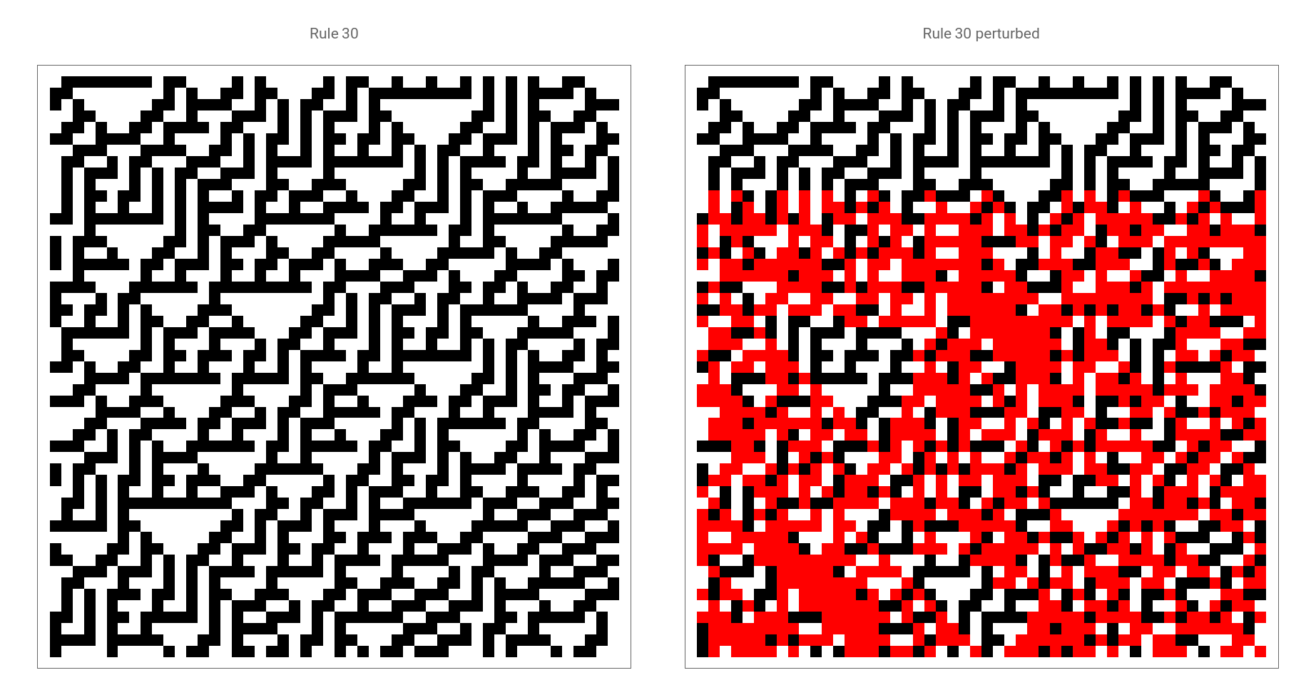
As an example consider the evolution of the famous rule 30 which displays class 3 behaviour. Suppose we want to introduce a slight perturbation in the evolution of the CA above. We can perturb the system by inputting that only at state 10 it should act as a rule 90 cellular automata, while the subsequent evolutions return to applications of rule 30 (the cells that evolve differently after the perturbation is applied are colored red):
As an example consider the evolution of the famous rule 30 which displays class 3 behaviour. Suppose we want to introduce a slight perturbation in the evolution of the CA above. We can perturb the system by inputting that only at state 10 it should act as a rule 90 cellular automata, while the subsequent evolutions return to applications of rule 30 (the cells that evolve differently after the perturbation is applied are colored red):
Out[236]=
Out[238]=

n-Flip Perturbations
n-Flip Perturbations
More specific to the project problem, we define a function called nFlipCA which performs n-cell flips (i.e. color changes from white to black and vice versa) for a given rule at a given iteration time. The scope is to apply this function once the knowledge about which cells to perturb is obtained. As before, we highlight in red every cell which is different from the normal evolution after the perturbation is applied:
In[65]:=
nflipCA[rule_,init_,t_,fun_,position_,tsub_]:=If[position=={},CellularAutomaton[rule,init,t],If[tsub==0,CellularAutomaton[rule,fun[CellularAutomaton[rule,init,{{{tsub}}}],position],t],Module[{newstate=fun[CellularAutomaton[rule,init,{{{tsub}}}],position]},Join[CellularAutomaton[rule,init,tsub-1],{newstate},CellularAutomaton[rule,newstate,{{1,t-tsub}}]]]]]
As an example, let us swap the color of the middle cell for rule 30 at time 25 during the evolution of 50 cells:
Out[76]=
Rule 30: Unperturbed (left) vs Pertubed (right) |
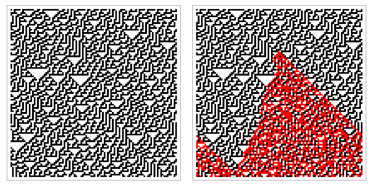
Notice how the light cone (and thus the limit at which the information of the perturbation travels) extends clearly from the perturbed middle cell: due to the boundary conditions it, also, passes through the right “wall” of the cellular automata and affects the left hand side.
Considering the Problem Within Linear Cellular Automata
Considering the Problem Within Linear Cellular Automata
Finding the Kernel of Linear Rules
Finding the Kernel of Linear Rules
Considering elementary cellular automata, there exist only 8 linear/additive rules: {0, 60, 90, 102, 150, 170, 204, 240} [4]. Linear automata behave analogously to linear systems, in particular their overall evolution can be expressed as a linear combination of individual evolutions, where the additive operations is specific to the rule chosen. In mathematical terms, additive automata require that the evolution of arbitrary states α and β upon application of the rule satisfies , where the symbol denotes the additivity operation of the rule chosen [5]. Exploiting the similarity with linear systems, we can express a linear rule as a linear combination of its “basis” states, i.e. states where only one cell is black/active, while the remaining cells are set white:
L
L(α⊕β)L(α)⊕L(β)
⊕
In[77]:=
basisAutomata[rule_,n_]:=Transpose[CellularAutomaton[rule,#,{{{1}}}]&/@Permutations[PadRight[{1},n]]]
For rule 90, the 6-cell basis states evolve as follows:
Out[21]=
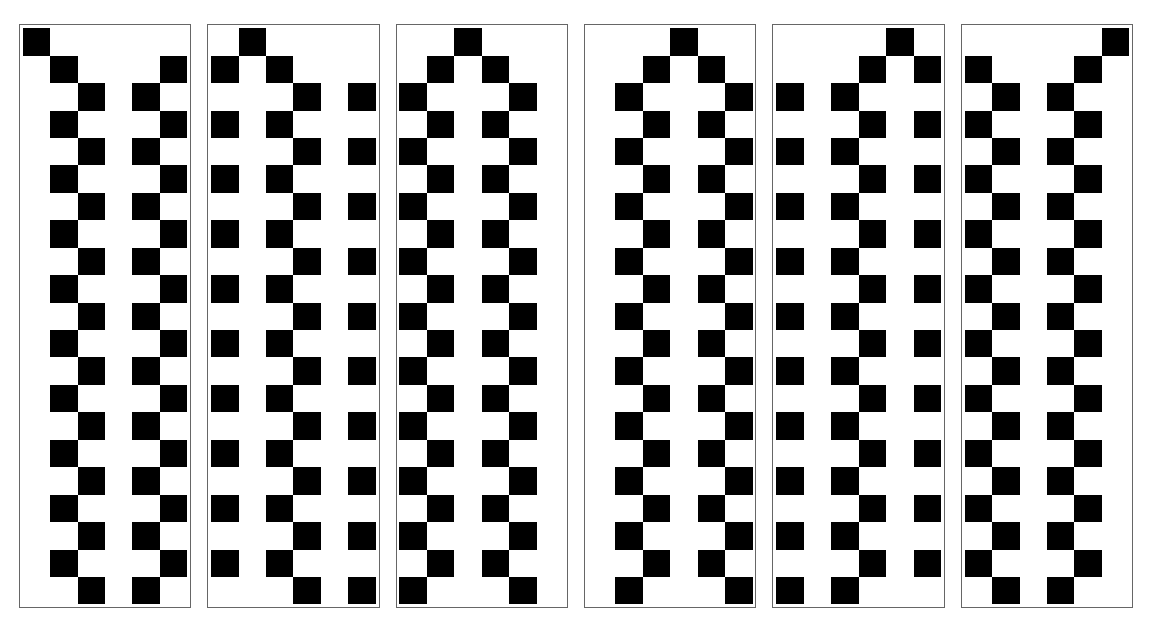
Notice how the basis states evolve in the same way, they only get shifted (a resemblance of the fact that the propagation operator is shift invariant).
By exploiting the tools of Linear Algebra, the evolution of the basis states for the case above can be cast in matrix form representing the rule transformation as
Out[19]//MatrixForm=
0 | 1 | 0 | 0 | 0 | 1 |
1 | 0 | 1 | 0 | 0 | 0 |
0 | 1 | 0 | 1 | 0 | 0 |
0 | 0 | 1 | 0 | 1 | 0 |
0 | 0 | 0 | 1 | 0 | 1 |
1 | 0 | 0 | 0 | 1 | 0 |
Given a number of cells in 1D, finding the states for which the evolution leads to a zero state is now equivalent to finding the kernel of the transformation rule for some powers with , where we can improve the efficiency of this function by adding the constraint that the computations should stop when the kernel of is found equal to the kernel of , as we assume that the kernel for higher powers won’t change anymore. Additionally, since many states appear multiple times in the kernel of higher matrix powers, we thus remove these duplicates from the final set of kernels:
ncell
n
L
n
n≤
ncell
2
n
L
n+1
L
In[78]:=
solveKernel[rule_,ncell_,npower_,nsolutions_]:=Module[{varlist=Table[Unique["x"],{ncell}]},(varlist/.#)&/@FindInstance[MatrixPower[Transpose[CellularAutomaton[rule,#,{{{1}}}]]&/@Permutations[PadRight[{1},ncell]],npower].varlist==ConstantArray[0,ncell],varlist,nsolutions,Modulus2]]
Considering the linear rule 90, we can display some of these states belonging to the null space of the rule transformation:
Out[83]=
Some Rule 90 Null Space States |

Solving for Linear Cellular Automata
Solving for Linear Cellular Automata
We found an analytical method to explore the kernel of linear cellular automata and thus find the states which map to zero after a certain number of iterations. The task now is to implement an algorithm/function that given any initial condition manages to find the minimum amount of the cells to perturb so that the cellular automata will map to zero by using the knowledge of the states contained in the null space of the linear rule.
In[84]:=
swapFunctionLinearAutomata[rule_,init_,t_]:=Module[{kernel=kernelwoduplicate[First@solvekernelstop[rule,Length[init],100000]]},Module[{nearestf=Nearest[Catenate@kernel->All,DistanceFunctionHammingDistance]},Module[{firstpositionsmall=Ordering[#["Distance"]&/@Catenate[nearestf[CellularAutomaton[rule,init,t]]],1]},Module[{positionswap=Catenate@Position[Mod[(#["Element"]&/@Catenate[nearestf[CellularAutomaton[rule,init,t]]])[[First@firstpositionsmall]]-CellularAutomaton[rule,init,{{{First@firstpositionsmall-1}}}],2],1]},If[First@firstpositionsmall-1<0,CellularAutomaton[rule,init,t],nflipCA[rule,init,t,funswap,positionswap,First@firstpositionsmall-1]]]]]]
We can test the function for the whole range of additive elementary rules (as usual, the red cells correspond to the perturbations applied):
Considering the Problem Within Non-Linear Cellular Automata
Considering the Problem Within Non-Linear Cellular Automata
Dynamical System Approach
Dynamical System Approach
It comes without a surprise that the nonlinear case is fundamentally more complicated to solve, and in the end we will see that it comprises to the fact that computational irreducibility does not allow us to know in advance which states drive the cellular automata to a zero state.
The approach followed consists, firstly, in defining a so called attractive surface containing the set of states that map to zero after n- steps for a given rule. We introduce the terminology n-iter dimension to specify that the n-iter dimensional attractive surface for a given rule is comprised of states that evolve to a zero entropy state in 1 up to n iterations.
We will now consider the simplest case of 1-iter dimensional attractive surfaces:
As an example, the states in the attractive surface for rule 20 and for 4 cells are given by:
A clean and effective way to display these states is by plotting the state transition diagrams:
For instance, consider the state diagram of all the states for rule 20 and 4 cells (where the zero state has been labelled by “0”):
For instance, consider the state diagram of all the states for rule 20 and 4 cells (where the zero state has been labelled by “0”):
From the diagrams above, it can be clearly seen that some states remain disconnected from the attractive surface, and thus this will prevent them to spontaneously evolve to the zero state. It thus follows that the state transition diagrams give a nice visual formulation of the problem in question: acting as a Maxwell Demon, the task is to define a procedure which takes states not connected to the zero states and perturbs them so that they eventually enter the attractive surface. We now have the goal to study and analyze the behaviour of these disconnected state, and eventually learn when to perturb them at the right time and positions during the evolution of the cellular automata.
A visual example of the procedure explained is given below, where for rule 20 and 4 cells one state outside the attractive surface is perturbed to reach the zero state:
A visual example of the procedure explained is given below, where for rule 20 and 4 cells one state outside the attractive surface is perturbed to reach the zero state:
Hamming Entropy
Hamming Entropy
For instance, considering rule 51 with 3 cells, the state {0,0,1} evolves for 5 steps as follows:
We can extract the Hamming distances only:
Study of Typical Behaviour
Study of Typical Behaviour
For instance, considering rule 30 for 10 cells, the states outside of the attractive surface display an intricate behaviour (each state is represented by a line of different color):
For graphical ease, a less cluttered plot is shown for rule 30 and 7 cells:
The behaviour shown it’s interesting: for this particular configuration most of the states do oscillate periodically with an amplitude of either 2 bits or 1 bit but never enter the attractive surface.
Following on this, we select some rules belonging to the four Wolfram classification and analyze how states tend to evolve with respect to the attractive surface.
As expected, states evolving according to the class 1 rules we analyzed reach the attractive surface spontaneously, as characterized by their global uniform behaviour. Nevertheless, we can see in the right graph that there exist some states that stabilize at a fixed Hamming distance although rule is of class 1. As an example take the state :
which indeed correspond to the non-uniform but periodic evolution
Notice that if we consider class 1 rule where the final pattern reaches black cells global consensus (such as rule 239 which is the black-white equivalent to rule 8) we obtain the opposite pattern, as the maximum Hamming distance from the zero state is indeed reached by the black state:
Analysis of class 2 rules that typically show periodic behaviour:
For class 2 rules most states tend to asymptotically stabilize at a fixed hamming distance/entropy from the attractive surface. This is reasonable as class 2 rules display periodic behavior, and as such the states get visually shifted along the cells as they evolve, but their bit difference/Hamming distance to the zero states is, indeed, unaffected.
We repeat the same procedure for class 3 rules:
We repeat the same procedure for class 3 rules:
Again, not surprisingly, class 3 rules display much more chaotic behaviour. It appears that after a brief complex transient response (where some states do also manage to enter the attractive surface) the states seems to eventually oscillate periodically. A similar phenomenon is shown below by the entropic evolution of class 4 rules:
Notice in these case how some states also show metastable behaviour, that is they get closest to the attractive surface but then eventually drive away and stabilize at a fixed Hamming distance.
Additionally, we can infer how it seems that rules not always tend to evolve states to the highest entropy/distance possible. While this phenomenon may seem intuitive for class 1 and class 2 rules, the pattern seems to apply surprisingly also at class 3 and 4 rules. It is conjectured thus that only a modest percentage of rules does evolve states to the maximum distance possible. We can easily test this for the whole range of elementary rules up to 10 cells:
It appears that as the number of cells increases only about 1/3 of the rules evolve to states at maximum entropy from the attractive surface.
Solving the Problem for the General Case
Solving the Problem for the General Case
Knowing which states do map to zero for a given rule and number of cells, we can now implement a function that, given an initial state and an evolution time, it checks which state(s) within the evolution come closest to the states in the attraction surface. It thus then applies the necessary perturbations to this state in order to drive the cellular automata to a zero entropy state.
As a nice example consider the evolution of rule 54 for 15 cells.
Displaying these with the aid of transition diagrams, the perturbation applied looks as follow:
Having defined the necessary functions to study and perturb effectively the evolution of the cellular automaton to the zero state, we can test it on a range of rules and initial conditions. This part is displayed in the appendix for formatting ease of the project. Here we show two applications of the function to rule 54 and 30 and 16 cells:
Generalization to Arbitrary Attractive Surface Iter-Dimensions
Generalization to Arbitrary Attractive Surface Iter-Dimensions
We display a nice application of this general function for rule 54 and random initial condition on 10 cells where the zero state is achieved by the minimum perturbation possible, i.e. changing one cell bit only.
In the appendix, many applications of this general perturbation function for different n-iter-dimensional attractive surface are shown.
Computational Implications of the Perturbation Procedure
Computational Implications of the Perturbation Procedure
Concluding remarks
Concluding remarks
The project consisted of defining a procedure to perturb the evolution of a cellular automaton in order to drive it to a zero entropy state with the minimum effort required, effectively acting as refrigerator system. The task was divided by first considering the simpler case of additive cellular automata, where by exploiting the tools of linear algebra it was possible to define a function that accurately solved the problem. The next step was to analyze more general rules, and by introducing the concept of Hamming distance and attractive surface, a perturbation function was again developed to artificially affect the evolution of the system to reach a zero entropy state. Although excellent results were achieved upon application of the function, for the general case, it was not possible to work on registers of size higher than 20-30 cells due to the excessive computational effort required. It was argued that this was a more general instance of the principle of computational irreducibility leading to an eventual lack on information of what perturbations to choose.
Following on the work done, other possible paths of investigation could consist of carrying these perturbation ideas to an application of the Knuth-Bendix algorithm for rewriting systems, where the perturbations applied would be interpreted as performing Knuth-Bendix completions to reach local confluence on a graph and test it its thermodynamical consequences.
Following on the work done, other possible paths of investigation could consist of carrying these perturbation ideas to an application of the Knuth-Bendix algorithm for rewriting systems, where the perturbations applied would be interpreted as performing Knuth-Bendix completions to reach local confluence on a graph and test it its thermodynamical consequences.
Keywords
Keywords
◼
Cellular Automata
◼
Thermodynamics
◼
Perturbations
◼
Computational Irreducibility
Acknowledgment
Acknowledgment
During the time at the 2022 Wolfram Summer School, I had the possibility to engage and converse with a wide range of great people. In particular, I am grateful to Stephen Wolfram for introducing me to this project and the feedback provided during the course of the School. I am also vastly thankful to both my mentors Jon Lederman and Tom Lee for their constant support, help and time dedicated to me and the project. Additionally, I acknowledge and deeply thank Jonathan Gorard for his lectures from which I learned considerably, the exciting daily conversations we had and his invaluable comments that helped shaped the project and the directions pursued. Finally, I must thank all the splendid mentors and students I met during the great time at the Summer School.
References
References
◼
[1] Wilks, J. (1971). The Third Law of Thermodynamics, Chapter 6 in Thermodynamics, volume 1, ed. W. Jost, of H. Eyring, D. Henderson, W. Jost, Physical Chemistry. An Advanced Treatise, Academic Press, New York, page 477.
◼
[2] S. Wolfram, “Cellular automata as models of complexity”, Nature 311:419 (1984).
◼
[3] J. Salem and S. Wolfram, Thermodynamics and hydrodynamics with cellular automata, inTheory and Applications of Cellular Automata, S. Wolfram, ed. (World Scientific, 1986).
◼
[4] S. Wolfram, “A New Kind of Science”, 2002, Wolfram Media, Champaign, IL, https://www.wolframscience.com/nks/notes-6-5--additive-cellular-automaton-rules/
◼
[5] S. Wolfram, “A New Kind of Science”, 2002, Wolfram Media, Champaign, IL, https://www.wolframscience.com/nks/notes-6-5--generalized-additivity-in-cellular-automata/
◼
[6] S. Wolfram, "A New Kind of Science", 2002, Wolfram Media, Champaign, IL, https://www.wolframscience.com/nks/p444--irreversibility-and-the-second-law-of-thermodynamics/