ABSTRACT(original article): In this paper, we derive a series of exact analytical closed expressions to calculate the complex eigenfrequencies and the displacement for the corresponding eigenmodes of a viscoelastic (nano)sphere in the presence of linear damping. Where possible, we provide closed expressions for damping rates, including the contributions from viscosity, as well as thermal conductivity and solutions of the heat equation. We assume an isolated system, such that no energy/heat transfer to the environment is allowed. We find monotonic behavior of the damping as a function of frequency for breathing and torsional modes, however, for spheroidal modes we find non-monotonicity. Furthermore, we analytically analyze the thermodynamic limit for all mode types. We also investigate the frequency shift and find expected behavior, i.e., a reduced eigenfrequency with damping than without damping for breathing and torsional modes. For spheroidal modes, however, we find non-monotonic shifts, corresponding to the damping. For some eigenfrequencies, we find anomalous frequency shifts. CITATION (original article): Markus Wenin, Andreas Windisch, “Vibrations and damping of the eigenmodes of viscoelastic nanospheres with thermal conductivity”, Archive of Applied Mechanics, Volume 95, 122 (2025), https://doi.org/10.1007/s00419-025-02830-7
Introduction
Introduction
This Mathematica Notebook (written in Version 14.3) is based on our paper Vibrations and damping of the eigenmodes of viscoelastic nanospheres with thermal conductivity, [1]. In order to obtain the correct results, the cells below have to be evaluated in order. In principle, most of the content can be evaluated on a standard desktop computer, even though the evaluation of some computations may take several minutes. Cells that contain parameters that can be changed are marked like this. The notebook is structured in three sections. The first section focuses on breather modes, the second section on spheroidal modes, and the third section on torsional modes.
Parameters and definitions
Parameters and definitions
Auxiliary calculations
Auxiliary calculations
Breather modes
Breather modes
Now that we have defined all relevant quantities, we will discuss the three mode types individually below.
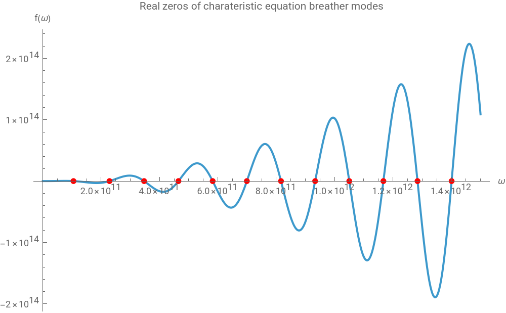
Let us start by computing the real eigenfrequencies for breather modes.
ω$breath$table=NSolveValues[{fbreath[ω,0,0]==0,0<ω<1.510^12},ω,WorkingPrecision->30];ShowPlot[fbreath[ω,0,0],{ω,0,1.510^12},AxesLabel{"ω","f(ω)"}],ListPlot[Thread[{ω$breath$table,0ω$breath$table}],PlotStyle->Red],
Out[]=
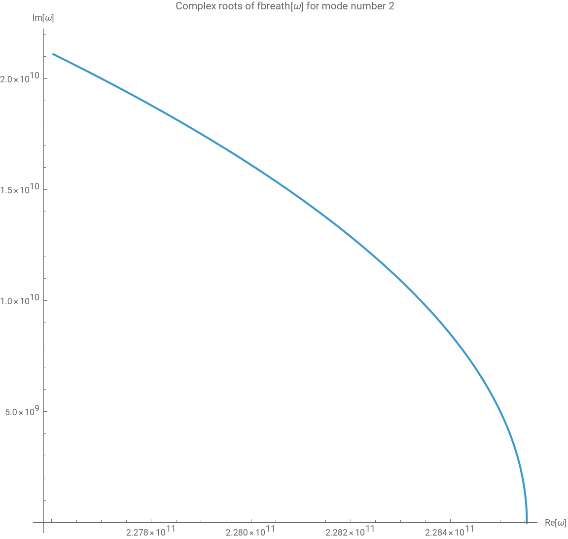
Once the real roots have been obtained, we can determine the roots for varying η1 and for a given mode number mode$num.
mode$num=2
;ω$eta$breath$list[η1s_,η2s_,ωstart_]:=ω/.(FindRoot[fbreath[ω,η1s,η2s],{ω,ωstart},MaxIterations->20000,AccuracyGoal->30,WorkingPrecision->70])η1max=1/10;nmax=50;dη1=η1max/(nmax-1);η1tab=Table[dη1*(i-1),{i,1,nmax}];w=Table[0,{nmax}];ωstart=ω$breath$table[[mode$num]];Do[ωi=ω$eta$breath$list[dη1*(i-1),(-2dη1(i-1)/3),ωstart];ωstart=ωi;w[[i]]=ωi,{i,1,nmax}];rootplot=ComplexListPlotw,Out[]=
Next, we define the various formulae for the decay rate γ, obtained through different approaches and for fixed values of η1 and η2.
(*viscousandthermaldampingcoefficientsbreathermodes*)γvisc$diff$breath=Simplify[I(η1(D[fbreath[ω,η1s,η2s],η1s]/.η1s->0/.η2s->0)+η2(D[fbreath[ω,η1s,η2s],η2s]/.η1s->0/.η2s->0))/(D[fbreath[ω,η1s,η2s],ω]/.η1s->0/.η2s->0),Assumptions->cl>0];γvisc$int$breath=-(8η1+8η1-4η1-2η2+8(-1+)η1Cos[2klR]+klR(2(-8+)η1+η2)Sin[2klR])(2ρ(-2+2+2Cos[2klR]+klRSin[2klR]));γvisc$asympt$breath=(2η1+η2)ω^2/(2ρcl^2);γT$breath[ω_]=kconstTv^2;
2
kl
2
R
4
kl
4
R
4
kl
4
R
2
kl
2
R
2
kl
2
R
2
kl
2
R
2
R
2
kl
2
R
4
kl
2ρT0
2
ω
Out[]=
n | 1 | 2 | 3 | 4 | 5 | 6 | 7 | 8 | 9 | 10 | 11 | 12 |
frequency ω 0 | 106 | 228 | 348 | 464 | 582 | 700 | 816 | 934 | 1050 | 1168 | 1284 | 1400 |
frequency Re[ ω | 106 | 228 | 348 | 464 | 582 | 698 | 816 | 932 | 1050 | 1166 | 1282 | 1398 |
frequency ω asympt | 106 | 228 | 348 | 464 | 582 | 698 | 816 | 932 | 1050 | 1166 | 1282 | 1398 |
Out[]=
n | 1 | 2 | 3 | 4 | 5 | 6 | 7 | 8 | 9 | 10 | 11 | 12 |
γ visc ω -6 10 s | 152 | 2110 | 5256 | 9650 | 15298 | 22198 | 30352 | 39762 | 50424 | 62342 | 75514 | 89940 |
γ visc -6 10 s | 152 | 2110 | 5256 | 9650 | 15298 | 22198 | 30352 | 39762 | 50424 | 62342 | 75514 | 89940 |
γ visc -6 10 s | 152 | 2110 | 5256 | 9650 | 15298 | 22198 | 30352 | 39762 | 50424 | 62342 | 75514 | 89940 |
γ visc -6 10 s | 508 | 2402 | 5540 | 9930 | 15576 | 22476 | 30630 | 40038 | 50702 | 62618 | 75790 | 90218 |
γ T -6 10 s | 2212 | 10456 | 24118 | 43240 | 67822 | 97866 | 133372 | 174340 | 220772 | 272666 | 330020 | 392840 |
In[]:=
surface$breath$plot[t_]:=ParametricPlot3D[Re@(R+Exp[Iω$breath$table[[1]]t]ubreath[R,ω$breath$table[[1]],η1,η2][[1]]){Sin[θ]Cos[ϕ],Sin[θ]Sin[ϕ],Cos[θ]}/.Al->0.1,{θ,0,Pi},{ϕ,0,2Pi},PlotRange->{{-1.1R,1.1R},{-1.1R,1.1R},{-1.1R,1.1R}}];
In[]:=
Monitor[ListAnimate[Table[surface$breath$plot[t],{t,0,2Pi/ω$breath$table[[1]],1/502Pi/ω$breath$table[[1]]}]],t]
Out[]=

Spheroidal modes
Spheroidal modes
Let us start by computing the real eigenfrequencies for spheroidal modes for a given mode number n$num.
n$num=2
;(*n$num>=1,casen$num=0reducestobreathermodes,n$num=1correspondstoanunphysicaltranslatorymode,seediscussionin[3]*)m$num=1
;(*-n$num<=m$num<=n$num*)ω$spher$table=NSolveValues[{fspher[n$num,ω,0,0]==0,0<ω<5.510^11},ω,WorkingPrecision->30];ShowPlot[fspher[n$num,ω,0,0],{ω,0,5.510^11},AxesLabel{"ω","f(n,ω)"}],ListPlot[Thread[{ω$spher$table,0ω$spher$table}],PlotStyle->Red],Once the real roots have been obtained, we can determine the roots for varying η1 and for a given mode number freq$num and mode number n$num set above.
Next, we define the various formulae for the decay rate γ, obtained through different approaches and for fixed values of η1 and η2.
Evaluation of this cell may take some time . n$plots defines how many plots will be produced covering one period in equitemporal steps (starting at 0, and excluding 2 π/ω) .
Torsional modes
Torsional modes
Once the real roots have been obtained, we can determine the roots for varying η1 and for a given mode number freq$num$tors and mode number n$tors set above.
Next, we define the various formulae for the decay rate γ, obtained through different approaches and for fixed values of η1 and η2.
References
References
◼
[1] Markus Wenin, Andreas Windisch, “Vibrations and damping of the eigenmodes of viscoelastic nanospheres with thermal conductivity”, Archive of Applied Mechanics, 95, 122 (2025), https://doi.org/10.1007/s00419-025-02830-7
◼
[3] Eringen, A.C., Suhubi, E.S.: Elastodynamics, “Linear Theory, vol. II”, Academic Press, New York (1975)
CITE THIS NOTEBOOK
CITE THIS NOTEBOOK
Vibrations and damping of the eigenmodes of viscoelastic nanospheres with thermal conductivity
by Andreas Windisch, and Markus Wenin
Wolfram Community, STAFF PICKS, May 8, 2026
https://community.wolfram.com/groups/-/m/t/3713420
by Andreas Windisch, and Markus Wenin
Wolfram Community, STAFF PICKS, May 8, 2026
https://community.wolfram.com/groups/-/m/t/3713420