Abstract. Defective vertex colorings were introduced in 1986. Unlike proper vertex colorings they allow a fixed number of the neighbors of a vertex v to have the same color as v. We introduce an efficient computational method for finding defective colorings of a finite graph that runs in polynomial time.
Introduction
Introduction
The usual definition of a vertex coloring in graph theory requires that adjacent vertices (vertices that share an edge) receive different colors. In the 1980s relaxations of this definition were introduced and studied. One, called “defective coloring” allows a fixed number of vertices adjacent to a vertex v in the graph to have the same color as v (see [ 2 ]). One application is to allocation of shared resources(say, use of a computer network) at different times (represented by different colors) among users (the vertices) having competing needs (as shown by edges). What level of competition (size of defect) is acceptable? Many papers have been written and are still being written on these colorings.Cowen, Goddard and Jesurum[ 5 ], outlined a method for finding certain defective colorings in polynomial time. We shall implement this method, in Mathematica, for 3-colored graphs. An additional purpose of this post is to show how graph vertex coloring can be used to do research in Mathematica.
Definitions
Definitions
A graph G = < V, E> consists of a set V called vertices and a set E of unordered pairs of elements of V, called edges. In this paper we will assume that all graphs are finite, that is, V is a finite set. A function c: V ⟶ {1, 2, ..., k} will be called a k-coloring of the graph G; c is a proper k-coloring if { ,}∈E implies that c() ≠ c(). The neighborhood of a vertex v, N( v ), consists of all vertices in V that share an edge with v, that is, N( v ) = { w ∈ V | { v, w } ∈ E }. The number of elements or cardinality of N( v ) will be denote by |N( v )|. A graph G = < V, E> is (k, u) colorable, where k is a positive integer and and u is a non-negative integer, if there is an k-coloring of G such that for any v ∈ V, at most u members of N( v ) have the same color as v. Obviously a proper k-coloring is the same as an (k, 0) coloring. The mixing number of a k-colored graph G is the number of edges whose vertices receive different colors.
v
1
v
2
v
1
v
2
Let c be a k-coloring of G. Then a vertex v ∈ V will be called k-secure under c if more than |N(v)| of the vertices in N(v) are colored with the same color as v; otherwise it will be called k-insecure. A k-coloring c will be called k-insecure if every vertex is k-insecure. We note that insecure 2-colorings were known as unfriendly 2-colorings in [ 1] and [5]. If k is fixed, we drop the "k" and just use "secure" and "insecure."
1
k
Main Results
Main Results
The first result we wish to establish is that every finite graph G = < V, E> has a k-coloring that is insecure. The basic idea can be seen from the following example. Suppose the vertices of G have been colored with three colors: red, blue and green and G has a red vertex v with five red and three blue and one green neighbor. Then v is a secure vertex, since it has 9 neighbors, 5 of which are red, and 5 > (1/3)(9).
In[]:=
reds={1,2,3,4,5,6};blues={7,8,9};greens={10};WheelGraph[10,VertexLabelsAutomatic,VertexStyleFlatten@{#Red&/@reds,#Blue&/@blues,#Green&/@greens}]
Out[]=
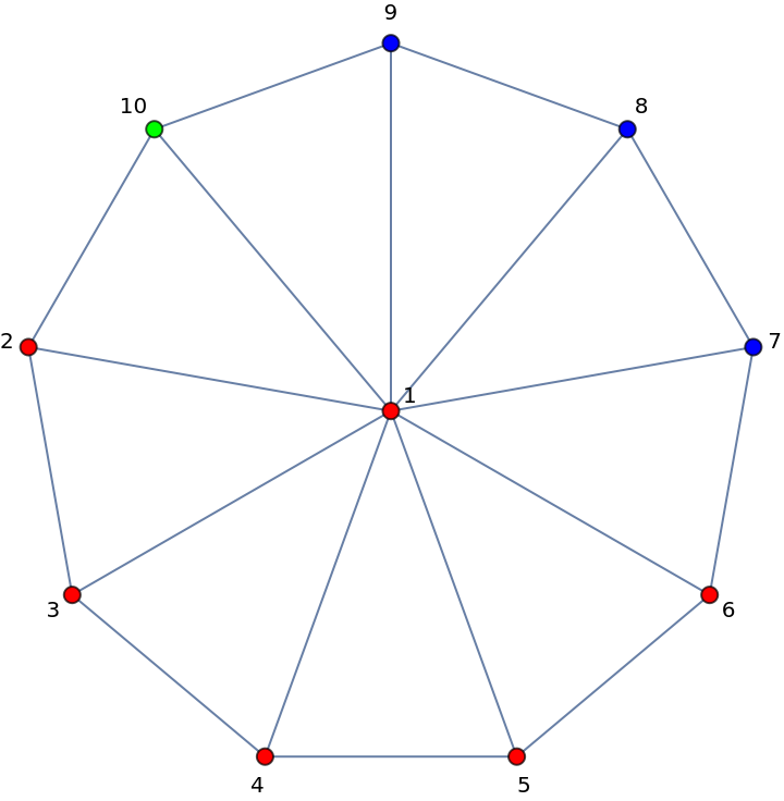
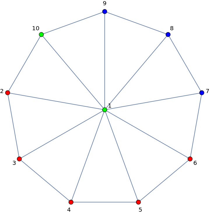
If we change v's color to green then v would now be insecure since 1 < (1/3)(9). Note that this change has increased the mixing number of G (by +4)as well. Thus, the basic idea is to find secure vertices and change them as shown to insecure vertices; since the mixing number increases, but is bounded (by the number of edges), this process must terminate with all vertices being "insecure."
In[]:=
reds={2,3,4,5,6};blues={7,8,9};greens={1,10};WheelGraph[10,VertexLabelsAutomatic,VertexStyleFlatten@{#Red&/@reds,#Blue&/@blues,#Green&/@greens}]
Out[]=
Theorem 1. Let G = < V, E> be a finite graph. Then G has a insecure k-coloring. Proof. Suppose that G has a k-coloring and under this coloring v is a secure vertex. Then more than |N(v)| of the vertices in N(v) are colored with the same color as v. Hence there must be some color i, where 1 ⩽ i ⩽ k, such that fewer than |N(v)| of the vertices in N(v) have color i; for, if not, there would be (k-1) colors, each with at least |N(v)| of the vertices in N(v) having these colors and one color (v’s color) having more than |N(v)| vertices, in N(v). However, then there would be more than |N(v)| vertices in N(v)!
1
k
1
k
1
k
1
k
Now, if we change v's color to i, it would increase the mixing number of the graph (since only the edges that have one vertex v and the other vertex in N(v) would be affected) . In this way we can successively eliminate secure vertices. Since the mixing number is bounded by the number of edges in G, this process surely terminates in a finite number of steps leaving only insecure vertices, that is, an insecure k-coloring. ■
In [ 5 ] an argument is given that the above procedure of eliminating secure vertices runs in O(E×Δ) time, where E is the number of edges and Δ is the maximum degree in G.
The following theorem is well known (see [5], [6]) and follows easily from Theorem 1 as we now show.
Theorem 2. Let G be a finite graph with n vertices with maximum degree Δ(G). If 2 ⩽ k < n, then any insecure k-coloring of G is a (k, ⌊Δ(G)/k⌋)-coloring of G where ⌊u⌋ is the greatest integer less than or equal to u.
Proof. Theorem 1 implies there is an insecure k-coloring c of G.Then at most (1/k)|N(v)| vertices
in N(v) have the same color as v under coloring c. But |N(v)| ⩽ Δ(G), for all vertices v of G; so
(1/k)|N(v)| ⩽ (1/k) Δ(G) = Δ(G)/k. However, the number of vertices in N(v) having the same color as v is an integer; therefore, at most ⌊Δ(G)/k⌋ vertices adjacent to v have the same color as v under the coloring c.
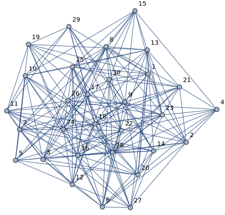
Next, we consider a rather large example. The following list of edges, E200, was created with the RandomGraph function and has 30 vertices and 200 edges.
In[]:=
E200={12,18,19,113,116,117,119,120,123,125,127,129,130,24,26,28,29,213,214,216,217,218,221,227,228,36,37,38,39,310,311,312,317,320,322,325,326,328,414,415,420,421,422,423,426,428,57,510,512,516,517,519,520,522,526,528,530,69,612,614,616,620,622,624,626,627,628,630,78,79,710,711,712,714,716,718,724,725,726,89,813,815,817,821,822,824,825,826,830,911,914,915,918,920,921,923,929,1011,1013,1015,1016,1018,1024,1025,1026,1028,1029,1116,1118,1119,1124,1126,1127,1128,1129,1216,1217,1218,1221,1223,1224,1225,1227,1230,1314,1315,1318,1319,1320,1321,1323,1325,1328,1330,1416,1420,1424,1427,1428,1429,1430,1517,1523,1525,1526,1530,1617,1618,1619,1620,1622,1623,1625,1627,1718,1719,1723,1724,1725,1726,1727,1729,1820,1821,1823,1824,1825,1827,1828,1829,1924,1926,1929,1930,2023,2024,2026,2027,2123,2124,2125,2128,2130,2223,2224,2225,2226,2228,2229,2230,2324,2326,2328,2426,2526,2528,2628,2630,2728,2830};
We display this graph below.
In[]:=
g200=Graph[E200,VertexLabelsAutomatic]
Out[]=
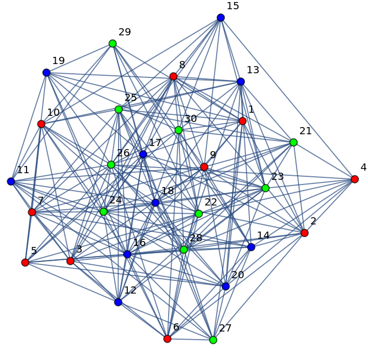
We arbitrarily color the first 10 vertices red, the next 10, blue, and the last 10, green.
In[]:=
reds=Range[10];blues=Range[11,20];greens=Range[21,30];
To display the colored graph we introduce the following function.
In[]:=
graph[r_,b_,g_][G_]:=Graph[G,VertexLabelsAutomatic,VertexStyleFlatten@{#Red&/@r,#Blue&/@b,#Green&/@g}]
We display next, the vertex-colored graph.
In[]:=
graph[reds,blues,greens][E200]
Out[]=
What is the color of vertex 6? red. What constitutes “red”? For us “red” is the set of all vertices “colored red”, that is the set, “reds.” Same for other colors. So a “coloring” can be thought of as a partition of the vertices of the graph.
To change the color of a vertex means to move it from one set of the partition to another. If it is in set “x” and we want to move it to set “y”, we need to delete it from set x, using DeleteCases and then add it to set y using Append. Say, we want to change the color of vertex 6 from red to blue.
Now vertex 6 is blue and not red. We redraw the graph with this change.
We restore the original coloring.
An edge is called mixed in the colored graph if its end vertices have different colors.
The mixing number of a vertex-colored finite graph is the number of edges with different colored endpoints. Certainly this number is bounded by the number of edges of the graph.
For example, here are the neighbors of vertex 3 in E200.
For example we show that vertex 13 is blue and secure.
So 13 is blue and has 5 blue neighbors and 5/14 > 1/3; thus vertex 13 is secure. However, vertex 20 is blue but insecure.
So vertex 20 has 14 neighbors, 4 of which are blue and 4/14 is less than 1/3. So vertex 20 is blue but insecure.
The next function,whatcolor, labels the color of a vertex as either "red", "blue", or "green", depending upon whether it is in reds, blues, or greens.
Here is the original coloring.
Next, we introduce SercureVertexQ, which tests for secure vertices in a 3-colored graph.
Next, we again restore the original coloring.
Thus vertex 2 is red and secure. Here are the neighbors of vertex 1.
We now need to find their colors; that is, what sets of the color partition they belong to. The function NeighborColors[ i ] defined below maps the color function whatcolor onto the set of neighbors of vertex i will do this for us.
In order to count the various colors, we use Tally.
It can occur that some color or colors are missing from the colors of the neighbors of a vertex, v. To capture this in general we introduce the function MissingColor.
We need a function that gives the color that occurs least often(maybe not at all!) in the neighborhood of a vertex. We introduce two functions LeastFrequentColor and FirstMinColor[ ] to do this.
The next function, FirstMinColor selects the color that occurs least often in the neighborhood of a vertex v (if some colors do not occur at all, it returns the first of those).
Now vertex 2 is red and is secure with green as the minimum color in its neighborhood. If we changed 2’s color to green, it would increase the mixing number of the graph.
The next function, ChangeColor, looks at the neighborhood of a vertex v and selects the color that occurs least often(maybe not at all) and changes v’s color to that color. It is easy to see that this will increase the mixing number of the colored graph--if there are any secure vertices!
Insecure Coloring Program
Insecure Coloring Program
We initialize again.
The following short program produces an insecure 3-coloring starting with any 3-colored finite graph.
Here is an insecure 3-color partition of our graph starting with the original coloring.
If we use this coloring, there will be no secure vertices.
We display the “insecure” coloring of this graph.
Defective 3-coloring the graph
Defective 3-coloring the graph
We now turn to the problem of finding a defective 3-coloring of our graph g200. We want to apply Theorem 2, so we need to know the maximum degree of the graph, Δ(G). We use VertexDegree to find the 30 vertex degrees of the graph.
An inspection shows that its Maximum Degree, Δ(G) = 18 and ⌊18/3⌋ = 6. So G is (3, 6)-colorable, by Theorem 2. The insecure 3-coloring in Figure 6 was found, starting with our initial coloring, in less than half a minute, on a MacBook Air laptop. Note that 6 is an upper bound; hence, it might be (3, u) colorable for u < 6.
The following calculation shows that the above coloring of the graph is in fact a (3, 5)-coloring, but not (3, 4)-coloring. For each vertex i, it counts the number of vertices in the neighborhood of i, that have is color. We see that this always less than or equal to 5. Whether the graph itself is (3, u)-colorable for u < 5 has not been determined.
We could find another insecure coloring starting with another initial coloring, say, all red vertices.
This insecure coloring is a (3 , 4) - coloring of our graph, as the following calculation shows. Maybe other insecure colorings will lead to even better defective colorings; however we have not pursued this further.
Acknowledgments
Acknowledgments
We thank Lenore Cowen for pointing out that the algorithm presented runs in O(E×Δ) polynomial time, where E is the number of edges and Δ is the maximum degree in graph G. We also thank George Beck for improvements in coding and style throughout.
References
References
1) R. Aharoni, E. C. Milner and K. Prikry, Unfriendly Partitions of a Graph, Journal of Combinatorial Theory, Series B, 50(1), 1990 pp. 1–10. https://doi.org/10.1016/0095-8956(90)90092-E.
2) L. Cowen, R. Cowen, and D. Woodall, Defective colorings of graphs in surfaces: partitions into subgraphs of bounded valence. Journal of Graph Theory , 10, 187 - 195, 1986.
3) R. Cowen, “Mixing Numbers and Unfriendly Colorings of Graphs,” The Mathematica Journal, 2021. doi.org/10.3888/tmj.23–4.
4) R. Cowen and W. Emerson, “Proportional Colorings of Graphs,” 1985, unpublished, but cited in [ 1 ].
5) L. Cowen, W. Goddard, C. Jesurum. Coloring with Defect, SODA ‘97: Proceedings of the eighth annual ACM-SIAM symposium on Discrete algorithms January 1997 Pages 548–557.
6) M. Frick and M. Henning, Extremal results on defective colorings of graphs, Discrete Mathematics, 126, 151-158. 1994.
Conclusion
Conclusion
Defective Colorings have become an important topic in graph theory but little has been done computationally to find them. We have tried to remedy that by implementing the suggested method of [ 5 ] in Mathematica. Although we only consider 3-colorings, it should be clear how to extend to more “colors.”
In the future it would be worthwhile to develop a program that inputs a k, for k colors and then produces the desired defective k-coloring.
In the future it would be worthwhile to develop a program that inputs a k, for k colors and then produces the desired defective k-coloring.