For additive elementary cellular automaton rules such as rule 90, the period of the space-time diagonal at depth m, read mod a prime p, multiplies by p exactly when m crosses a power of p. This essay asks how far that pattern extends across the whole elementary rule space. I scan all 256 nearest-neighbor rules empirically with FindTransientRepeat applied to full light-cone diagonals, under a strict confirmation criterion that rejects repeats living only in the tail of the observation window, and I cross-check the measurements against an exact algebraic framework built from three ingredients: (i) the diagonals of every additive rule are columns of a q-nomial coefficient triangle, whose periods mod p follow exactly from Lucas' theorem and the Frobenius endomorphism; (ii) every rule whose left neighbor enters its algebraic normal form linearly obeys a cumulative-sum recurrence along diagonals, which forces all its diagonal periods to be powers of p times a small background factor; (iii) a unique "binomial spectrum", obtained by inverting the Pascal matrix mod p, measures how far any diagonal is from the additive core. The scan then sorts the rule space cleanly: mod 2, not a single rule shows a confirmed period that is not a power of 2. 146 rules have eventually constant diagonals, 81 have bounded power-of-2 periods, 25 show unbounded power-of-2 growth with doubling pinned to powers of 2 for the additive core, and 4 rules (30, 45, 75 and 135) double so fast, roughly once per depth step, that every finite window is eventually exceeded – consistent with the Fibonacci-size dependency of the rule 30 columns established and verified below.
Introduction
Introduction
An elementary cellular automaton (ECA) evolves a row of cells by a rule that maps each neighborhood of three cells to a new cell value. Started from a single nonzero cell, the evolution paints the familiar space-time triangles: rule 90 draws the Sierpinski gasket, rule 30 draws an apparently random texture, rule 110 draws interacting localized structures.
Instead of reading that picture row by row, this project reads it along diagonals of slope 1: the sequence of values seen by an observer who moves one cell to the right at every time step. The diagonal at depth m starts at position -m at time 0 and crosses the entire light cone. Diagonals are natural for two reasons. First, information in a radius-1 automaton propagates one cell per step, so a slope-1 line is a causal boundary: the depth-m diagonal is driven only by the two diagonals above it. Second, for additive rules the diagonals turn out to be exactly the columns of Pascal-like coefficient triangles, which makes their periodic structure fully computable.
The starting point is a system of binomial-style recurrences I developed for rule 30, written out in full in the next section: the columns of the rule 30 pattern along its center and its two edges obey Pascal-like bracket recurrences, and the n-th term of the k-th column is determined by the first F(k+2) terms of that column, where F(k+2) is the (k+2)-nd Fibonacci number. This project is linked to the following questions:
1
.Investigate patterns from combinations of binomial coefficients and polynomials modulo k.
2
.Catalog patterns produced by combinations of integer functions modulo k.
3
.Study the periodicities on diagonals of the rule 30 pattern modulo m.
4
.Study code 10.
5
.Find an explicit formula for the cell color in rules 225, 45, 30.
6
.Investigate Fibonacci modulo n.
7
.Search for mathematical constants with regularities in their digit sequences.
This essay attacks the third question, generalized from rule 30 to the entire elementary rule space: which rules show the slow, power-of-p period growth of the additive family as depth grows, which saturate or freeze, and which produce something else? The method combines an empirical scan (FindTransientRepeat on every diagonal of every rule, with an explicit robustness check on the observation window) and an exact framework (the recurrence system, a cumulative-sum doubling mechanism, the multinomial-column theorem, and the binomial spectrum).
The mathematical framework this essay runs on – the diagonal recurrence system and its telescoping, the multinomial (q-nomial) column theorem for additive rules, the binomial spectrum, and the general decomposition machinery that expands any diagonal in a basis formed by multinomial-coefficient columns or by the diagonals of any other rule – is developed in full, with complete proofs and in greater generality, in the author's paper "Unified Theory of Deterministic Cellular Automata (UTOCA)" [6], https://doi.org/10.5281/zenodo.21306383. The theorems below state those results in the form needed here and specialize them to the period-classification question; the companion paper is the reference for every mathematical aspect beyond that.
Behind the binomial spectrum sits a more general idea used throughout: decomposition from any basis to any basis, over any modulus. Fix a modulus M – prime or composite – and any family of reference sequences: the columns of a q-nomial coefficient triangle, or the diagonals of any other elementary rule taken in the same centered form. Whether and how a given diagonal expands as a Z_M-linear combination of that family is a finite linear-algebra question, solvable by gcd-based elimination even when M has zero divisors; the answer is a coefficient set whose size, stability as the observation window grows, and residual weight measure how much of one rule's behavior is visible through another rule's algebra. Periods are one invariant of a diagonal; its coefficients in another rule's basis are a second, finer one. The classification carried out in this essay is the special case in which the reference basis is Pascal's triangle.
Setup: mod-p rules and full light-cone diagonals
Setup: mod-p rules and full light-cone diagonals
Every ECA rule number encodes a Boolean function of three bits. Writing that function in algebraic normal form (ANF: XOR of AND monomials) and reading XOR as + and AND as × turns the rule into a polynomial over the integers, which can be reduced mod any modulus p. For p = 2 this reproduces the standard rule exactly; for p > 2 it defines a canonical mod-p lift of the same rule, acting on cell values 0, ..., p-1.
From a rule number to its mod-p polynomial rule:
Out[]=
Mod[#1+#3,2]&
The evolution is computed on the full two-sided light cone, positions -size to +size, so that every diagonal is complete from t = 0. This matters: truncating the picture to positions ≥ 0 silently deletes the first m terms of the depth-m diagonal, and those initial terms carry transient structure that the period detector needs to see.
Full-cone evolution from a single seed cell, and its slope-1 diagonals:
Out[]=
{0,0,0,0,1,1,1,1,0,0,0,0,1,1,1,1,0,0,0,0}
A space-time plot with one diagonal highlighted:
Out[]=
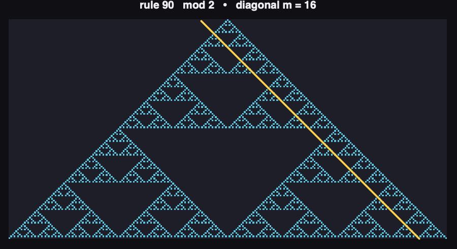
Reading the figure: the nested empty triangles of the rule 90 gasket are the geometric face of the Frobenius identity Q(y)^(2^L) = Q(y^(2^L)) mod 2 – every doubling of scale reproduces the whole pattern with gaps. The highlighted line is the depth-16 diagonal: it enters at the apex offset 16 positions to the left, crosses every scale of the fractal once, and samples exactly the 8-th column of Pascal's triangle mod 2 (Theorem 6 below). The long empty stretches it crosses are the zero digits forced by Lucas' theorem, and the periodic bursts it picks up are what FindTransientRepeat will measure as a period-16 cycle.
Diagonals as recurrent sequences
Diagonals as recurrent sequences
Write D_m(t) for the value on the depth-m diagonal at time t, i.e. the cell at position t - m. Because each cell depends on its three upper neighbors, and those neighbors sit on diagonals m, m-1 and m-2 at time t-1, every rule f induces the same triangular system of recurrences:
D
m
D
m
D
m-1
D
m-2
where the first argument of f is the left neighbor. The diagonals with negative depth lie beyond the light cone, where the row is spatially uniform; the uniform background value cycles under v ↦ f(v, v, v), with some period c (for quiescent rules c = 1; for rules with f(0,0,0) ≠ 0 the whole background flashes, e.g. c = 2 for rule 165 mod 3). This background period is the seed of the small non-p factors observed later.
Definition 1 (left-linear rule). A rule is left-linear mod p when its ANF polynomial has the form f(l, c, r) = l + g(c, r) mod p: the left variable appears as a lone linear term and in no product.
Exactly 16 of the 256 rules are left-linear mod 2 – including rules 30, 45, 75, 135 and the whole additive family:
Out[]=
{15,30,45,60,75,90,105,120,135,150,165,180,195,210,225,240}
Theorem 1 (telescoping).
Theorem 1 (telescoping).
For a left-linear rule, subtracting consecutive terms of the diagonal recurrence eliminates f and leaves D_m(t) - D_m(t-1) = g(D_(m-1)(t-1), D_(m-2)(t-1)), so each diagonal is the running sum of a function of the two diagonals above it:
D
m
D
m
t-1
∑
j=0
D
m-1
D
m-2
Proof: immediate by induction on t. ■
The rule 30 column system and its Fibonacci dependency
The rule 30 column system and its Fibonacci dependency
For rule 30 the triangular system takes a form worth writing out in full, because it supports two exact results that anchor the fast end of the classification. Fibonacci numbers enter through their binomial summation form:
Definition 2 (Fibonacci).
F
k+2
F
k+1
F
k
k+1
∑
j=0
k-j+1 |
j |
Reading the rule 30 pattern along its center column and along its two families of diagonals defines three bracket symbols, each satisfying a binomial-style recurrence mod m obtained by translating rule 30's polynomial f(l, c, r) = l + c + r + c·r into the corresponding coordinate frame:
Definition 3 (rule 30 center columns).
n |
k |
C
n-1 |
k+1 |
C
n-1 |
k |
C
n-1 |
k-1 |
C
n-1 |
k+1 |
C
n-1 |
k |
C
Definition 4 (rule 30 left columns).
n |
k |
L
n-1 |
k |
L
n-1 |
k-1 |
L
n-1 |
k-2 |
L
n-1 |
k |
L
n-1 |
k-1 |
L
Definition 5 (rule 30 right columns).
n |
k |
R
n-1 |
k |
R
n-1 |
k-1 |
R
n-1 |
k-2 |
R
n-1 |
k-1 |
R
n-1 |
k-2 |
R
The right system is precisely the slope-1 diagonal system of this essay: comparing Definition 5 with the general diagonal recurrence shows (n over k)_R = D_k(n) for rule 30, term by term – the same-column symbol enters linearly (that is rule 30's left-linearity), and the product couples only the two columns above.
The bracket recurrence reproduces the rule 30 diagonals exactly (True):
Out[]=
True
Theorem 2 (rule 30 telescoped). Because the same-column symbol is linear, Theorem 1 collapses the whole n-recurrence of the right columns into a single sum over the two previous columns:
n |
k |
R
n-1
∑
j=0
j |
k-1 |
R
j |
k-2 |
R
j |
k-1 |
R
j |
k-2 |
R
Proof: Theorem 1 applied to Definition 5, with the empty base column (0 over k)_R = 0 for k ≥ 1. ■
Numerical check of Theorem 2 (True):
Out[]=
True
Theorem 3 (Fibonacci dependency). For n ≥ F(k+2), the n-th term of the k-th right column of rule 30 is determined by the first F(k+2) terms of that column, through the binomial interpolation:
n |
k |
R
F
k+2
∑
p=1
F k+2 |
k |
R
n-1 |
F k+2 |
F k+2 |
p |
p+1
(-1)
F
k+2
F
k+2
The formula reconstructs the whole column from its first F(k+2) values – the effective memory of the k-th diagonal is Fibonacci-sized, growing like the golden-ratio power ϕ^k. (For n < F(k+2) the summand p = F(k+2) - n degenerates; those n are exactly the initial data.)
Numerical check of Theorem 3 for k ≤ 6, F(k+2) ≤ n ≤ 40 (True):
Out[]=
True
Proposition 4 (cumulative-sum period growth)
Proposition 4 (cumulative-sum period growth)
Let s(j) be eventually periodic with period P and let S(t) be its running sum mod p. Over one period the sum advances by the constant block sum σ = Σ s(j) over a period. If σ = 0 mod p then S is eventually periodic with period P; otherwise S(t + P) = S(t) + σ and, since p is prime, p blocks are needed to return: the period is exactly pP. In both cases period(S) ∈ {P, pP}. ■
Corollary 5 (all periods of left-linear rules are p-powers).
Corollary 5 (all periods of left-linear rules are p-powers).
By induction up the triangular system: the background diagonals are periodic with the small period c, and each new diagonal multiplies the joint period of the two above it by at most p (Proposition 4 applied to Theorem 1). Hence for every left-linear rule, every eventually periodic diagonal has period dividing c · . Mod 2, where c ≤ 2, every confirmed diagonal period of rules 15, 30, 45, 60, 75, 90, 105, 120, 135, 150, 165, 180, 195, 210, 225, 240 must be a power of 2 – no other period length is possible, no matter how chaotic the picture looks. The scan below confirms this without a single exception, and the affine rules mod 3 show precisely the background factor c = 2 (periods 2·3^j).
(m+1)
p
What Proposition 4 does not fix is the rate: it allows the period to multiply by p at every depth step, but says nothing about when it actually does. The two extremes both occur. For the additive rules the multiplication happens only when the depth crosses a power of p (Theorems 6-8 below): the doubling depth grows exponentially, the period grows only logarithmically in m. For rule 45 the scan measures a doubling at nearly every step – Proposition 4 saturated. Theorem 3 places rule 30 in between: when the effective memory of a column grows like ϕ^k, period doubling per O(1) depth steps is available, and the measured rate of roughly one doubling per two depth steps matches that exponential dependency.
Measuring periods
Measuring periods
FindTransientRepeat[seq, 3] splits a sequence into a transient prefix and a block that repeats at least 3 times. Used naively it has a failure mode that matters here: on a diagonal whose true period exceeds the window, it can classify almost the whole window as "transient" and certify a tiny accidental repeat found in the last few entries. The cure is a strictness condition: a period only counts as confirmed when the transient occupies at most half the window, so the repeating part is actually observed over a substantial stretch.
Strict period measurement (period 0 means: nothing confirmed in this window):
Out[]=
{1,1,2,1,4,1,4,1,8,1,8,1,8,1,8,1,16,1,16,1,16,1,16,1,16,1,16,1,16,1,16,1,32}
The strictness condition is not pedantic – it changes an answer. In a 700-step window, the depth-14 diagonal of rule 45 appears to lock into period 3: FindTransientRepeat reports {period 3, transient 692}, i.e. a 9-element repeat squeezed into the tail of the window. Widen the window to 2500 steps and the truth appears: the same diagonal has period 512 with no transient at all. The "period 3" was noise; rule 45 is actually still doubling.
The same diagonal of rule 45, seen through a 700-step and a 2500-step window:
Out[]=
{700{period3,transient692},2500{period512,transient0}}
Rule 45 with the wide window: a doubling cascade with no end in sight (0 = beyond even this window):
In[]:=
Table[diagPeriod[caDiagonal[45, 2, 2500, m]], {m, 0, 20}]
Out[]=
{2,4,8,8,16,32,32,64,64,128,128,128,128,256,512,512,512,512,512,512,0}
Reading the output: periods 2, 4, 8, 8, 16, 32, 32, 64, 64, 128, 128, 128, 128, 256, 512, ... – rule 45 multiplies its diagonal period by 2 roughly once per depth step, the fastest growth Proposition 4 permits. Any fixed window is exceeded at a depth proportional to its logarithm; a scan must treat such rules as a class of their own rather than trust whatever the tail of the window happens to show.
Largest confirmed period up to depth m (log base 2), for four representative rules:
Out[]=
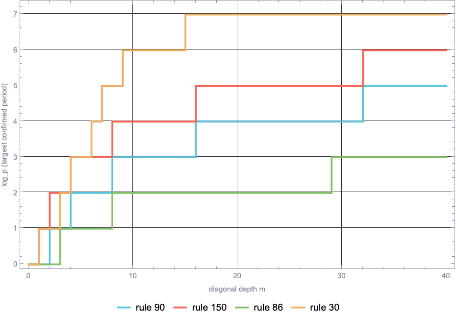
Reading the plot, curve by curve. Rule 30 (orange) climbs a staircase of slope about 1/2: one doubling every two depth steps, period roughly 2^(m/2) – the exponential regime of Theorem 3; it hits 2^7 by depth 15 and the 700-step window certifies nothing beyond. Rule 150 (gold) rises by exactly one unit at m = 1, 2, 4, 8, 16, 32: doubling exactly at the powers of 2, period 2^⌈log2(m+1)⌉ – the logarithmic regime of Theorem 7. Rule 90 (blue) is the same staircase delayed by a factor 2 (its depth-m diagonal is the Pascal column k = m/2, and odd diagonals are empty). Rule 86 (green) creeps: three doublings in forty depths. All four are power-of-2 staircases – they differ only in how often they climb, which is exactly what the classification below has to capture.
The additive core
The additive core
Additive rules evolve by polynomial powers
Additive rules evolve by polynomial powers
A rule is additive mod p when its local map is linear: α·left + β·center + γ·right mod p. Mod 2 these are the XOR rules 0, 60, 90, 102, 150, 170, 204, 240. Encode a row as a generating polynomial; one time step multiplies it by αy + β + γ/y, so from a single seed the whole field consists of the coefficients of the powers of one fixed polynomial.
Theorem 6 (diagonals of additive rules are coefficient-triangle columns).
Theorem 6 (diagonals of additive rules are coefficient-triangle columns).
For an additive rule with coefficients α, β, γ and single-cell seed, set Q(y) = γy² + βy + α. Then:
Proof. With A(y,t) = Σ a_j(t) y^j one has A(y,t) = (αy + β + γ/y)^t, so a_j(t) = [y^(t+j)] R(y)^t with R(y) = αy² + βy + γ. On the diagonal j = t - m this is [y^(2t-m)] R^t, and reading the coefficients of R^t backwards replaces R by its reciprocal Q(y) = y² R(1/y). ■
Rule 90 gives Q = 1 + y²: the diagonals are Pascal columns, D_2k(t) = Binomial[t, k] mod p, odd diagonals empty. Rule 150 gives Q = 1 + y + y²: the trinomial triangle columns.
Numerical check of Theorem 6 for rules 90 and 150 (both True):
Why additive periods jump only at powers of p
Why additive periods jump only at powers of p
Theorem 7 (column periods divide p^L).
Theorem 7 (column periods divide p^L).
Let Q over F_p have constant term 1 and T(t, k) = [y^k] Q(y)^t. If p^L > k then T(t + p^L, k) = T(t, k): the k-th column has period dividing p^⌈log_p(k+1)⌉. Proof: Frobenius gives Q^(p^L) = Q(y^(p^L)), so Q^(t+p^L) = Q^t · Q(y^(p^L)); extracting y^k, every term of Q(y^(p^L)) except the constant shifts by at least p^L > k and dies. ■ So for additive rules the period can jump only when the depth crosses a power of p – Proposition 4 restricted to its lazy extreme.
Theorem 8 (the binomial jump is exact).
Theorem 8 (the binomial jump is exact).
For k ≥ 1 the period of t ↦ Binomial[t, k] mod p is exactly p^L, L = ⌊log_p k⌋ + 1. Proof. "Divides" is Theorem 7. To rule out period p^(L-1): write k = d·p^(L-1) + r, 1 ≤ d ≤ p-1, 0 ≤ r < p^(L-1). Lucas gives Binomial[k, k] = 1. If d ≤ p-2, then k + p^(L-1) has digit d+1 at position L-1 and Lucas gives Binomial[d+1, d] = d+1 ≢ 1. If d = p-1 the addition carries, the digit becomes 0, and Lucas gives the factor Binomial[0, p-1] = 0. Either way the value moves. ■
Corollary (rule 90 mod p).
Corollary (rule 90 mod p).
The depth-2k diagonal has exact period p^(⌊log_p k⌋+1): the period multiplies by p exactly when m/2 crosses a power of p. Mod 2 this is the doubling staircase measured above; mod 3 the same staircase triples at powers of 3:
Rule 90 mod 3: period triples exactly when m/2 crosses 1, 3, 9, 27 (predicted: 3, 3, 9, 9, 9, ..., 27 from k = 9):
Reading the output: {1, 1, 3, 1, 3, 1, 9, 1, 9, ...} – odd depths are empty (period 1), and the even depths m = 2k carry period 3 for k = 1, 2, then 9 for k = 3 through 8, then 27 from k = 9: exactly p^(⌊log_3 k⌋+1). The additive core behaves identically at every prime, with p-fold jumps in place of doublings.
The binomial spectrum of an arbitrary diagonal
The binomial spectrum of an arbitrary diagonal
Theorem 6 covers the additive core. To probe every other rule with the same lens, invert the construction: instead of asking "which column is this diagonal?", ask "which combination of columns is this diagonal?". The Pascal matrix B[m, k] = Binomial[m, k] is lower triangular with unit diagonal, so det B = 1 and B is invertible over the integers mod any modulus. Every length-n sequence s therefore has a unique binomial spectrum c:
Theorem 9 (spectrum). For q = 2 the decomposition exists and is unique for every sequence and every modulus – a mod-M Newton forward-difference expansion. For q ≥ 3 (q-nomial columns) the powers Q^m have strictly increasing degrees, so a decomposition always exists over F_p, but uniqueness is lost. ■ The number of nonzero spectrum coefficients then measures distance from additivity: an additive diagonal is maximally sparse, a structureless one is dense.
The spectrum used here is the simplest member of a family: the companion paper [6] develops the decomposition against an arbitrary basis – any q-nomial triangle, or the diagonals of any other elementary rule taken in centered form, over any modulus, prime or composite – together with the solvability and uniqueness theory behind it. Everything computed in this section is the q = 2 specialization of that machinery. See https://doi.org/10.5281/zenodo.21306383.
Decomposition, reconstruction, and the rule 90 sanity check (a single term, c_8 = 1, for m = 16):
Spectrum sparsity by rule, along the first 40 diagonals:
Reading the plot: rule 90 (blue) sits at exactly one coefficient per nonempty diagonal – the diagonal is a Pascal column and the spectrum finds it. Rule 150 (gold) grows slowly and irregularly: its trinomial columns re-expanded in the binomial basis need a number of terms governed by the base-2 digits of m, still far below density. Rules 86 (green) and 30 (orange) saturate near half of all coefficients – the density expected of random sequences. The contrast between 86's near-flat period staircase and its dense spectrum is the important negative result here: eventual periodicity does not imply algebraic sparsity. Periods and spectra measure genuinely different kinds of order.
Scanning the full rule space
Scanning the full rule space
The scan computes the strict period profile of every rule from 0 to 255, seed {1}, window 700, diagonals m = 0 to 64, and sorts the profiles into five classes. "Constant": every confirmed period is 1. "p-power bounded": all confirmed periods are powers of p, none reaching p³. "p-power growing": powers of p reaching p³ or beyond. "Mixed": some confirmed period is not a power of p. "Window exceeded": at least half the diagonals confirm nothing – the fast-doubling regime.
The scan (about 3 minutes) and the classifier:
The growing class and the window-exceeded class:
Result (mod 2): 146 constant, 81 bounded, 25 growing, 4 window-exceeded – and the mixed class is empty. Not one of the 256 rules confirms a period that is not a power of 2. For the 16 left-linear rules Corollary 5 proves this; that the remaining 240 rules comply as well suggests the cumulative-sum mechanism reaches further than its hypothesis (rule 86, right-linear rather than left-linear, is the visible example). The growing class {18, 22, 26, 60, 82, 86, 90, 105, 124, 126, 129, 146, 149, 150, 154, 161, 165, 167, 181, 182, 193, 195, 210, 218, 225} contains the right-active additive rules 60, 90, 150, their affine complements (105, 165, 195, ...), and the nonlinear rules long known to emulate rule 90 on restricted configurations: 18, 22, 26, 82, 126, 146, 154, 182. The window-exceeded class {30, 45, 75, 135} is exactly the fast branch of the left-linear family: rule 30, its complement-conjugate 135, and the mirror pair 45, 75.
The same scan mod 3 (about 3 minutes):
Result (mod 3): the growing class is {18, 22, 26, 60, 82, 89, 90, 105, 123, 146, 150, 154, 182, 210, 218, 225}; the window-exceeded class is again exactly {30, 45, 75, 135}. The prime-independent core {18, 22, 26, 60, 82, 90, 105, 146, 150, 154, 182, 210, 218, 225} keeps its power-of-p growth at both primes; rules 89 and 123 join only mod 3. A large mixed class appears mod 3, led by the affine rules: rule 165 measures periods {2, 2, 6, 2, 6, 2, 18, 2, 18, ...} = 2·3^j with zero transients. The factor 2 is not noise – it is the background period c of Proposition 4: mod 3 the uniform background of rule 165 flashes 0 ↦ 1 ↦ 0 (since f(0,0,0) = 1, f(1,1,1) = 0), and every diagonal inherits that factor underneath its 3-power growth.
Elementary Cellular Automata
Elementary Cellular Automata
Plots
Plots
Data & Plots
Data & Plots
This section documents the full-scale scan behind the classification and the visual projections used to read it. The computation ran as a Wolfram Batch cloud job: for every rule 0-255, every enumerated seed index 2-20, and every modulus 2-20 – prime and composite – the strict period profile of the diagonals up to depth 64 was measured in an 800-step window. The result, periodData, is a single association keyed {rule, seed, modulus} whose values are the per-depth period vectors: about 92,000 profiles, six million measured periods. Every plot below is a projection of this one object along a different pair of axes. Two structural facts guide the reading. First, for composite modulus the ANF-lifted rule evolves compatibly with the Chinese remainder splitting of Z_m into prime-power components, so each diagonal period mod m is the lcm of its periods at the prime-power parts: moduli 6, 10, 12, ... contain no information beyond their prime-power factors and serve chiefly as consistency checks. Second, prime powers p^a with a ≥ 2 are genuinely new territory relative to the theorems of this essay – Lucas' theorem controls only a = 1 – so the mod-4, 8, 9, 16 slices are the empirical frontier, where the Zabek-style prime-power periodicity of binomial columns is the reference point [4].
Two scalar reductions compress each period vector to a single number. The saturation depth counts how many depth steps a profile keeps growing before it flattens – infinite when it is still climbing at the last measured depth – and is the scan's slow-doubling detector: additive rules saturate late and climb rarely (only when the depth crosses a power of p), constant rules saturate immediately, and the rule 30 family never saturates inside any finite window. The heatmap plots the final measured period over the rule × modulus grid: growing rules appear as hot horizontal bands, the prime-power columns carry the real structure, and each composite column reproduces the lcm of its prime-power parts, as the Chinese remainder argument predicts.
The doubling surface shows one rule at a time over the (depth, modulus) grid, with height log2 of the period, so every p-fold jump is a visible unit step. Additive rules produce terraced staircases whose treads lengthen geometrically – the three-dimensional shape of Theorems 7 and 8: jumps pinned to powers of p, tread length multiplying by p at each level. The rule 30 family produces steep ramps that hit the window ceiling; rule-86-type rules produce low, nearly flat terraces. The bar-chart variant renders the same integer data without surface interpolation, the honest choice when neighboring lattice points differ by an exact factor of p.
The last projection adds the initial condition as a third spatial axis: each point sits at (depth, modulus, seed), colored and sized by the log-period, one panel per rule. Seed-robustness of the classification appears as vertical uniformity of color along the condition axis. For additive rules that uniformity is a theorem: any finite seed is a superposition of translated single cells, a translated seed only re-indexes the diagonals, and a sum of p-power-periodic sequences is p-power-periodic – so the profile stays on the same skeleton for every seed, even where individual period values shift. Where a nonlinear rule's panel breaks the striping is precisely where its diagonal behavior genuinely depends on the seed; those (rule, seed) pairs mark the boundary of the seed-independent claims made in the findings.
Findings
Findings
Two growth regimes, one skeleton
Two growth regimes, one skeleton
Every nontrivial behavior found by the scan lives on the same skeleton – mod 2, all confirmed periods are powers of 2 – but the rules divide sharply by how fast they climb it. The additive core climbs logarithmically: Theorems 7 and 8 pin every jump to a power of p, so at depth m the period is only about m (rule 150) or m/2 (rule 90). The rule 30 family climbs linearly: rule 30 doubles about every two depth steps, rule 45 at almost every step, saturating the bound of Proposition 4. In between sits rule 86 with its barely-climbing staircase. Theorem 3 provides the structural reading of the fast regime: the k-th column of rule 30 carries a Fibonacci-sized memory of F(k+2) initial terms, growing like ϕ^k, and with exponentially growing memory a doubling per O(1) depth steps is available – rules 30 and 45 use it; the additive rules, whose memory is a single p-adic digit position, must wait for the next power of p.
Orientation matters: mirror pairs split
Orientation matters: mirror pairs split
Slope-1 diagonals probe the right-moving side of the light cone, so the classification is not mirror-invariant, and the splits are informative. Rule 30 (window exceeded) against its mirror rule 86 (2-power growing): the right diagonals of one are the left diagonals of the other, so this split says that rule 30 has a fast-doubling right edge and a slow-doubling left edge – the slow side being the well-known regularity of rule 30's left border, described by the left-column system of Definition 4. Rule 60 (growing) against its mirror 102 (constant): rule 102's activity leans entirely left, so every right-moving diagonal eventually exits its cone and freezes. Rules 45 and 75 mirror each other and both exceed the window: that pair is fast on both edges.
The mirror pair side by side:
Reading the figure: the two triangles are exact mirror images cell for cell. On the left picture (rule 30) the right edge is the turbulent side and a slope-1 diagonal dives straight into it; on the right picture (rule 86) the same geometric line runs along the quiet flank, picking up the near-periodic stripes that make its period staircase climb so slowly. Same automaton up to reflection, opposite diagonal physics.
Answer to the classification question
Answer to the classification question
Sorting all 256 elementary rules by the behavior of their diagonal periods mod p, with the strict window criterion, gives mod 2:
1
.146 rules: diagonals eventually constant. Includes every left-leaning mirror of a structured rule (102, 110, ...).
2
.81 rules: periods are powers of 2, bounded by 4 in the window – simple periodic backgrounds.
3
.25 rules: periods are powers of 2 and grow without visible bound. The additive rules and their affine complements double exactly at powers of 2 (Theorems 6-8); the rule 90 emulators (18, 22, 26, 82, 126, 146, 154, 182, ...) inherit the same staircase.
4
.4 rules (30, 45, 75, 135): periods double linearly in depth (about every one to two steps), provably powers of 2 by Corollary 5, but beyond confirmation of any fixed window past a logarithmic depth. What a naive scan reports as exotic mixed periods for 45 and 75 is a window artifact: at width 2500 the fake period 3 of rule 45 becomes a clean period 512 with zero transient.
5
.0 rules with genuinely mixed periods: mod 2 the p-power skeleton has no confirmed exception in the entire rule space.
Mod 3 the picture repeats with p-fold jumps, a prime-independent growing core of 14 rules, two mod-3-specific additions (89, 123), the same four window-exceeded rules, and a structural mixed class: the affine rules carry the extra background factor c = 2 predicted by Proposition 4, giving periods 2·3^j.
Concluding Remarks
Concluding Remarks
Reading elementary cellular automata along light-cone diagonals mod p turns "which rules are secretly additive?" into a decidable, quantitative question. Three exact mechanisms organize everything the scan sees: additive rules are multinomial-column automata whose periods jump exactly at powers of p; left-linear rules are cumulative sums whose periods can only multiply by p, at a rate anywhere between logarithmic and once-per-step; and the invertible binomial spectrum separates algebraic sparsity from mere periodicity. Empirically, mod 2, the entire rule space respects the power-of-2 skeleton without exception; the interesting axis is not which periods occur but how fast the doubling depth grows – logarithmic for the additive class and its emulators, linear for the rule 30 family, in agreement with the Fibonacci-size column dependency of Theorem 3.
The deeper concept the spectrum points at is basis-relativity: any diagonal of any rule can be interrogated in the basis of any other rule's diagonals, over any modulus, and the outcome is quantitative rather than rhetorical. A finite coefficient set that is stable under window growth means the target diagonal lies inside the basis rule's reachable class – for binomial columns mod p, exactly the purely periodic sequences with p-power period – while growing or unstable coefficients certify that the target's structure cannot be absorbed by that linear observer. In this language, "rule X emulates rule 90" becomes a rank statement about a change-of-basis matrix, and computational irreducibility becomes invariance of coefficient growth under every additive change of basis. Composite moduli add nothing mysterious: the Chinese remainder splitting Z_m into its prime-power components commutes with the polynomial rule map, so every decomposition question mod m factors into its prime-power parts. The companion paper [6] develops this decomposition calculus in full generality.
Three directions follow. First, prove the power-of-2 skeleton for the non-left-linear rules (rule 86's right-linearity suggests a mirrored telescope along the other diagonal direction, matching the left-column system of Definition 4). Second, turn Theorem 3 into a proven lower bound on the doubling rate of rules 30 and 45. Third, make the q ≥ 3 spectrum canonical by selecting the sparsest solution, so that "distance from additivity" becomes well defined at every prime, and check seed-independence of the whole classification over the enumerated finite seeds.
Acknowledgements
Acknowledgements
I thank my mentor Eric James Parfitt and Alejandra Ortiz Duran for guidance throughout this project, and the Wolfram Summer Research Institute staff, including Stephen Wolfram, thank you for your support.
Finally, my deepest thanks go to my son, Robert Nersissian, who remains my greatest source of inspiration and motivation.
Finally, my deepest thanks go to my son, Robert Nersissian, who remains my greatest source of inspiration and motivation.
References
References
1
.S. Wolfram (2002), A New Kind of Science. Wolfram Media.
2
.O. Martin, A. M. Odlyzko and S. Wolfram (1984), "Algebraic Properties of Cellular Automata," Communications in Mathematical Physics 93, 219-258.
3
.E. Lucas (1878), "Theorie des fonctions numeriques simplement periodiques," American Journal of Mathematics 1, 184-240.
4
.S. Zabek (1956), "Sur la periodicite modulo m des suites de nombres binomiaux," Annales Universitatis Mariae Curie-Sklodowska A10, 37-47.
5
.S. Wolfram (1984), "Universality and Complexity in Cellular Automata," Physica D 10, 1-35.
6
.T. Nersissian (2026), "Unified Theory of Deterministic Cellular Automata (UTOCA)," Zenodo. doi: https://doi.org/10.5281/zenodo.21306383
AI Disclosure
AI Disclosure
The following generative AI tools were used in this project: Claude Opus 4.8 (Anthropic), via Claude Code. It was used for developing and debugging the scanning and visualization code, cross-checking the proofs, and editing prose. All code and written content was reviewed, understood and approved by the author.
CITE THIS NOTEBOOK
CITE THIS NOTEBOOK
Classifying Cellular Automaton Rules by Diagonal Period Mod[p]
by Tigran Nersissian
Wolfram Community, STAFF PICKS, July 16, 2026
https://community.wolfram.com/groups/-/m/t/3763864
by Tigran Nersissian
Wolfram Community, STAFF PICKS, July 16, 2026
https://community.wolfram.com/groups/-/m/t/3763864