Wolfram Cloud Document

ABSTRACT (original article): Plant roots determine carbon uptake, survivorship, and agricultural yield and represent a large proportion of the world’s vegetation carbon pool. Study of belowground competition, unlike aboveground shoot competition, is hampered by our inability to observe roots. We developed a consumer-resource model based in game theory that predicts the root density spatial distribution of individual plants and tested the model predictions in a greenhouse experiment. Plants in the experiment reacted to neighbors as predicted by the model’s evolutionary stable equilibrium, by both overinvesting in nearby roots and reducing their root foraging range. We thereby provide a theoretical foundation for belowground allocation of carbon by vegetation that reconciles seemingly contradictory experimental results such as root segregation and the tragedy of the commons in plant roots. CITATION (original article): Ciro Cabal et al. ,The exploitative segregation of plant roots.Science 370, 1197-1199 (2020). https://doi.org/10.1126/science.aba9877
Computational supplement: SCIENCE 04 Dec 2020: Vol. 370, Issue 6521, pp. 1197-1199. DOI: 10.1126/science.aba9877
Featured in NEW YORK TIMES: How Selfish Are Plants? Let’s Do Some Root Analysis

Theoretical models are potent tools in ecology because they provide a mechanistic understanding of observed patterns, i.e., departing from the processes that underlie and drive them. This knowledge can ultimately generate well-informed hypotheses for the origin of those patterns. Analytical models are especially valuable because they rely on just a small subset of processes believed to be essential to explain an observed pattern. As a result, they are easy to analyze, and one can easily test the sensitivity of model predictions to changes in the parameters.

Our research developed a model to investigate how plants foraging soil resources respond to competition with other plants. It combined two ingredients that rarely appeared together in previous research: game theory to quantify plant responses to competition and explicit soil space. Using our model results, we generated hypotheses that were then tested qualitatively in a greenhouse experiment. In this entry, we describe our model briefly and provide Mathematica code to reproduce our main results. For a more detailed explanation, the reader may see the supplementary materials of the original article. We hope that this contribution fosters the use of Mathematica, even by beginners, as a potent tool to conduct ecological research.

Part 1. Predicting the spatial distribution of roots in solitary plants.

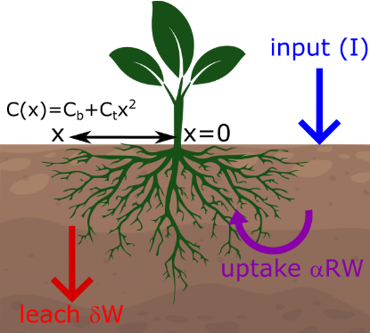
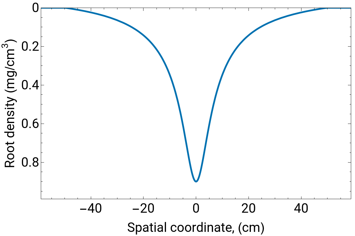
To understand how multiple plants compete with each other belowground, we first need to be able to predict the root foraging behavior of a plant growing alone. The root density distribution of a solitary plant should be used as ‘control’ to quantify the plant response to the presence of a neighbor. To produce this result, we first developed a basic spatially explicit model in which a plant is foraging a soil resource, W(x,t), through its its roots system, R(x,t). We implement a very simple soil resource dynamics in time (t) and space (x). At every spatial location, we assume that there is a fixed resource input (I) and a density dependent resource decay rate (δ W). We further assume that the ability of a plant to absorb resource from a soil location depends linearly on its root density at that location. Finally, the water absorbed by a given root density at a certain resource level is determined by a parameter (α) that defines a resource- and species-specific uptake rate (αWR). Based on this processes the dynamics for the resource follows Eq. [1],

[1]

Fig. 1. Schematic representation of the model processes.Developing and maintaining a root system has an obvious benefit for a plant because it allows her to obtain essential resources for survival and development. However, it also carries a cost (C) linked to the growth and maintenance of root tissues. In our model, we consider two types of roots, each with a different cost for the plant. First, fine roots are the local, low diameter, short-lived roots that absorb resources from the soil. The cost of these roots at a given location increases linearly with their density with a slope given by a parameter

. Second, coarse roots are structural, wide, lignified roots that connect the fine roots at any soil location with the point at which the plant stem touches the soil (x=0 in our model). The plant’s cost to grow these roots is highly spatially dependent because connecting the stem to fine roots will increase with the growing distance between both elements. For the sake of mathematical simplicity, we consider only one spatial dimension (x), and because we place the origin of coordinates at the plant insertion, x represents such distance. Based on basic hydraulics (i.e., modeling a coarse root as a hollow pipe and using Darcy’s Law to keep the flow inside the root constant), the relationship between distance and coarse root costs is well approximated by a quadratic growth. That is the cost scales with the square of the distance between the plant insertion point and the location of the fine roots. Putting together the costs associated to each class of roots, the total cost is C(x) =

Considering all the processes described above, and further assuming that resource dynamics is much faster than root growth and hence is in equilibrium at all times, we can calculate the local plant fitness. The local plant fitness is determined by the balance, in every soil location (independent from other soil patches), between the benefits of growing fine, absorptive roots and the cost of producing and maintaining both fine and coarse roots, Eq. [2].

[2]The optimal root density, i.e., the root density that maximizes plant fitness, is obtained when this balance is maximum. We calculate it from the partial derivative of G with respect to R and solving for R under the condition δG/δR = 0 and is shown below as OptR[x_]. The code in the next cell allows the reader to represent graphically such maximization for different parameter combinations.

Parameter values


Solution for a solitary plant

(*Extensionoftherootsystemofasolitaryindividual*)dc=

αi-Cbδ

Ctδ

;limit=IntegerPart[1.2*Abs[dc]];dx=2*limit/250;(*Optimaldistributionofrootdensityforasolitaryindvidual*)OptR[x_]:=Piecewise

δi

α(Cb+Ct

Abs[x]

)

,Abs[x]<dc,{0,Abs[x]>dc}(*Plotoftheresultsforinteractingindividuals*)PlotOptR[x],{x,-limit,limit},



Out[]=

Part 2. Predicting the spatial distribution of roots in pairs of competing plants.

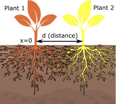
When two plants interact with each other, they may shift their behavior compared to when they are alone. While some plant roots can sense the identity of other roots they encounter (e.g. whether these other roots belong to another or the same individual, and even whether they belong to another species), in our model we explore the fundamental response of plants to the presence of a neighbor mediated by the changes in resource availability only. When individual 1’s roots encounter non-self roots from individual 2 in a soil patch, the resource decay rate in the soil patch will be exacerbated by those roots. In that soil patch, resource decay will be higher than the physical resource leach, proportionally to the root density of the second individual (R2) (see equation [3] reflecting the resource dynamics in a two plant scenario). In our model, plants will adjust their root density to such biotic exacerbation of the resource decay rate.

[3]In this new scenario, for each soil location x, we need to determine the root density of each plant of the pair,

and

. To this end, we can assume that the plant 1 is centered at x=0, and the plant 2 is centered at distance d from it. As we did for the solitary plant, we will only consider one spatial dimension for the sake of mathematical simplicity, and therefore the coordinate for plant 2 is x=d.

In this context, we can write the fitness-generating function for these two plants, as shown in the system of equations [4]:

[4]We use game theory to solve for the optimal strategy that plants may adopt in this new scenario. The conditions to solve these kind of problems in the context of evolutionary ecology is called the Evolutionary Stable Strategy (ESS). The ESS is generally expected to evolve by natural selection in natural populations. It gives the strategy a player would adopt if selfishly trying to maximize its own reward in a context in which all other individuals are adopting the same strategy. To obtain the ESS from our system of equations [4], we must calculate the partial derivatives of

as a function of

and of

as a function of

, and solve for

and

under the conditions

δG

δR

δG

δR

= 0. Derivatives are shown below as dG1 and dG2 (note that we used

rather than d to refer to the distance between the plants or the coordinate of plant 2). The next cells allow the reader to represent graphically such maximization and investigate its robustness to different parameterizations. It produces results for a solitary plant (table SampledSolitary), and then calculates the result for the two plants (tables T1 and T2). Note that this situation is harder to plot than the solution for a solitary plant. For a solitary plant, the root density is given by the piecewise solution OptR[x] plotted above. For the two-plant scenario, however, our model could allow the root density of a plant to respond to negative non-self root densities, which ecologically not possible. To properly represent the spatial distribution of root density, we need to define it as a piecewise function. To this end, we first draw the results as derived from the equations of the two plant-scenario [Eq. (4)] for all locations at which both

and

are positive. In all other points of the space if our model predicts negative

, we set it to zero and consider that plant 2 behaves as solitary hence predicting that its root density is given by OptR[x]. We follow this same rationale to determine

wherever the model predicts a negative

In the plot, the solitary plant root density centered in x=0 is represented with a blue dashed line. The interacting plant centered in x=0, or plant 1, is represented in orange. The main goal of our model is to compare the solitary plant (control) to a competing plant both centered in zero, and the difference between the interacting plant and the control quantifies the response to competition. In the plot, we also represent in yellow the neighbor (plant 2) with illustrative purposes.

Calculations to obtain the ESS equilibrium for a pair of competing individuals. The distance between plant insertion points is now a parameter (Fig. 1b in the main text).

Part 3. Total root production for different distances between plants.

In the previous parts of this notebook, we focused on the local responses of plants to competition with neighbors, which allowed us to determine the foraging range of each plant and the spatial root density distribution within that range. With these results, we predicted that plants respond to competition with neighbors by segregating their root systems, i.e., the foraging range shrinks in the direction facing a neighbor. However, another fundamental question root biologists and ecologists have been long interested in answering is how a plant should allocate its biomass among tissues to optimize its resources. A paradigmatic example of the resource allocation dilemmas plants face is represented by the belowground to aboveground allometry, or the root:shoot ratio. Previous game-theory models without an explicit description of the space have predicted that plants may engage in a belowground tragedy of the commons. A tragedy of the commons is a situation, often found in game-theoretical contexts, in which several players selfishly overexploit a shared resource pool (the commons) and reduce the total benefit the population gets from it. For plant roots, a tragedy of the commons occurs when competing plants allocate more into roots than if they were alone. Given that the total available resource is the same, plants increase their costs (more roots to build and maintain) while getting less benefit (less resource per plant). Following the above-mentioned model predictions, some experiments have confirmed that root overproduction happens at the expense of reproduction in interacting plants compared to solitary plants. However, these results have remained controversial for the last two decades, mainly due to problems with the experimental designs used to validate model predictions.

Our model provides a new, more realistic (spatially explicit) tool to test the optimal root allocation of plants and their response to interaction with other individuals. We used Mathematica to integrate the root densities for each plant in space from our previous model solutions to obtain a total root production. The integral of a root density (mg/cm) in space (cm) gives a weight (mg), which is indeed the total biomass of the root system of each plant. We can calculate this total root biomass for interacting plants at increasing distances. In the plot below, we compare the root biomass of a solitary plant (slashed grey line) with that of an interacting plant (orange curve) as a function of the distance (d) between them. Note that, of course, the solitary plant biomass remains unchanged with d. Remarkably, our results resolve the existing controversy by reconciling existing results. Our model shows that plants can respond to competition both overproducing (i.e., a tragedy of the commons) and underproducing roots! Moreover, the transition from one strategy to the other only depends on the distance between the plants, which agrees with previous studies predicting the tragedy of the commons only when plants are very close to each other, e.g., in very crowded plant populations.

CITE THIS NOTEBOOK

The exploitative segregation of plant roots
By Ciro Cabal, Ricardo Martinez-Garcia, Aurora de Castro, Fernando Valladares, Stephen W. Pacala
Wolfram Community, STAFF PICKS, April 1, 2021
https://community.wolfram.com/groups/-/m/t/2235435