Introduction to the problem. Urbanization demands advanced tools to analyze morphological changes caused by hostilities or disasters. This study bridges this gap by integrating artificial neural networks (ANNs) with LiDAR and GIS technologies, focusing on a site in Kharkiv, Ukraine, which was marginally impacted by the 2022 Russian invasion. Our key objective is to quantify urban resilience and transformation under extreme stress.
Review of previous works. Advances in CNNs and RNNs have enabled spatial-temporal analysis of LiDAR and multisource data. Recent methodologies improved feature extraction for urban change detection. However, gaps persisted in hostilities’ zone analysis, airborne and terrestrial LiDAR integration, and interpretability of ANN-driven insights.
Exposition of the main research material. Basics of ANNs for urban studies. This study employs two custom architectures: 1. ANN Similarity (Enhanced): A feedforward network using Mean Squared Error (MSE) loss and cosine similarity to predict dataset similarities. 2. Latest ANN Method: A deeper network with contrastive loss and Euclidean distance, emphasizing dissimilarity detection via convolutional/recurrent layers.
Applications in urban studies. The ANNs in this study were applied to the following from several listed industrial domains: 1. Routine Urban Monitoring: Detecting new constructions/demolitions in Tallinn, ESTONIA. 2. Hostilities Impact Analysis: Identifying war-induced structural changes in Kharkiv, UKRAINE. 3. 3D Feature Extraction: Automating building volumetry and change detection mapping from LiDAR point clouds.
Urban Remote Sensing with LiDAR. LiDAR’s millimeter-level accuracy enabled 3D modeling of urban features (e.g., building footprints, microtopography). Airborne (ALS) and mobile (MLS) LiDAR datasets were processed via proprietary iQ City Change Management (CCM) software, addressing challenges like ALS/MLS alignment and artifact filtering via point-density thresholds.
Case Study: urban change detection using LiDAR to assess hostilities’ impact. Methodology: the study analyzed multitemporal LiDAR datasets: Kharkiv (2019–2022): a 4 km² zone in Northern Saltivka, devastated by shelling. Tallinn (2017–2022): control datasets for routine redevelopment.
CCM Workflow: 1. Building Extraction (BE): identified structural features (Area, Volume, Height). 2. Change Detection (CD): classified changes as Added (new construction), Removed (demolition), or Unchanged.
ANN Analysis for comparing detected changes through Wolfram Mathematica: compared ANSE (similarity-focused) and LANN (dissimilarity-driven) methods. Results: The following changes detected. Kharkiv: 215 Added (pre-war redevelopment) and 51 Removed (war-induced demolitions) changes. The LANN method revealed stark contrasts (score: 0.35 and 0.32-0.42) between war-driven vs. routine redevelopment demolitions, capturing irregular demolitions. Tallinn: predictable redevelopment patterns (scores: 0.60-0.66 and 0.74), validating ANN accuracy for routine changes. Implications: LANN’s sensitivity to hidden features (e.g., structural degradation) gives policymakers detailed guidance for post-war recovery, and its divergence from statistical models highlights AI’s power to reveal unseen urban dynamics.
Conclusion. This research demonstrates how ANNs, fused with LiDAR/GIS, transcend traditional urban monitoring limitations. The framework offers scalable tools for disaster recovery, particularly in war zones.
CITATION (original article): Kostrikov Sergiy (2025). Analyzing urban morphology changes using neural networks. Visnyk of V.N. Karazin Kharkiv National University. Series Geology. Geography. Ecology, (62), 219-236. https://doi.org/10.26565/2410-7360-2025-62-17
Introduction
Introduction
This work concerns research on urban morphology in a city that experienced hostilities during 2022–2024. After lengthy negotiations, the municipality granted us permission to perform LiDAR monitoring in the most damaged area of Kharkiv. Because of the municipality’s IP restriction, I did not retain copies of the final source code. I only had a notebook with an earlier approach. It documents some initial stages of our ANN experiments in urban morphology, but it is far from the final results that were lost.
Left without the working source code, I had to implement a prompt Plan B and develop alternative tools to reproduce the published results. I’ll skip the longer introduction here - suffice to say it was possible only because I could build on the early entities; otherwise I could not have produced anything useful within a few days only….
A brief technical comparison of the two methodologies: my early attempt (the concluding part of which kept at the municipality) behaved partly like regression. The network’s output layer and loss function were not constrained to discrete class indices, so the model produced scalar or continuous outputs that I later interpreted; this caused rank/type mismatches. My enforced final approach is strictly classification-based: a 6-class Softmax output, explicit class index labels, and a cross-entropy loss, so predictions map directly and unambiguously to the six domain-defined categories. This final approach is implemented below.
1. Data Import & Preprocessing
1. Data Import & Preprocessing
This stage is all about getting the datasets ready for analysis. It starts by importing the source files, checking their structure, and making sure the feature values are standardized. Each dataset is handled separately to keep its unique variations intact, while also making sure they can all be compared on the same scale. This preprocessing step lays down a solid foundation for the modeling and interpretation that will follow.
baseDir="D:\\Wolfram_M\\ExampleData\\Combined\\CSV\\";files={"adjustedTestSetEST1nEST2nNEW.csv","adjustedTestSetEST1nKHNSnNEW.csv","adjustedTestSetEST2nKHNSnNEW.csv","adjustedTestSetEST1RnEST2RnNEW.csv","adjustedTestSetEST1RnKHNSRnNEW.csv","adjustedTestSetEST2RnKHNSRnNEW.csv"};classLabels={{"EST1n","EST2n"},{"EST1n","KHNSn"},{"EST2n","KHNSn"},{"EST1R","EST2R"},{"EST1R","KHNSR"},{"EST2R","KHNSR"}};
Robust per - file z - score normalization, column - wise
normalizePerFile[data_]:=Module[{cols},cols=Transpose[data];cols=Map[Function[c,With[{sd=StandardDeviation[c],m=Mean[c]},If[sd==0,ConstantArray[0,Length[c]],(c-m)/sd]]],cols];Transpose[cols]];
Import, validate first 6 numeric columns, normalize
preprocessedData=Table[Module[{path,raw,features},path=FileNameJoin[{baseDir,files[[i]]}];raw=Quiet@Import[path,"CSV"];If[!ListQ[raw]||raw==={},{},features=Select[raw,VectorQ[Take[#,6],NumberQ]&];If[features==={},{},normalizePerFile@N@features[[All,1;;6]]]]],{i,Length[files]}];
Table[{i,Length[preprocessedData[[i]]]},{i,Length[preprocessedData]}]
Out[]=
{{1,66},{2,68},{3,174},{4,24},{5,24},{6,87}}
2. Model Training (Classification)
2. Model Training (Classification)
In this phase, we train a predictive model to assess how similar two sets of features are . We carefully choose the network architecture and training parameters to strike a balance between accuracy and generalization . This way, the model can identify meaningful patterns in the datasets we’ ve prepared . The model we create becomes the analytical backbone for producing the similarity measures that will be used in the final evaluation
net=NetChain[{LinearLayer[64,"Input"->6],ElementwiseLayer[Ramp],DropoutLayer[0.3],LinearLayer[32],ElementwiseLayer[Ramp],LinearLayer[6],SoftmaxLayer[]},"Output"->NetDecoder[{"Class",Range[6]}]];
Clean rows so training data is never empty
cleanRow[row_]:=Replace[row,_?(Not@*NumericQ)->0,{1}];
Build training data from all rows (guaranteed length - 6 numeric)
trainingData=Flatten[Table[With[{row=cleanRow[preprocessedData[[i,j]]]},If[Length[row]==6,<|"Input"->Join[row[[1;;3]],row[[4;;6]]],"Output"->i|>,Nothing]],{i,Length[preprocessedData]},{j,Length[preprocessedData[[i]]]}],1];
Always train : with cleaned rows, trainingData is non - empty
trainedNet=NetTrain[net,trainingData,LossFunction->CrossEntropyLossLayer["Index"],MaxTrainingRounds->50,BatchSize->32,TargetDevice->"CPU",TrainingProgressReporting->"ProgressIndicator"];
simPredict=trainedNet;
3. Detected changes
3. Detected changes
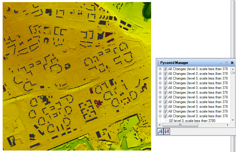
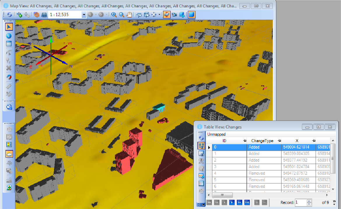
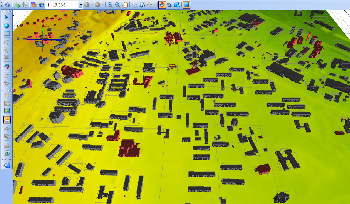
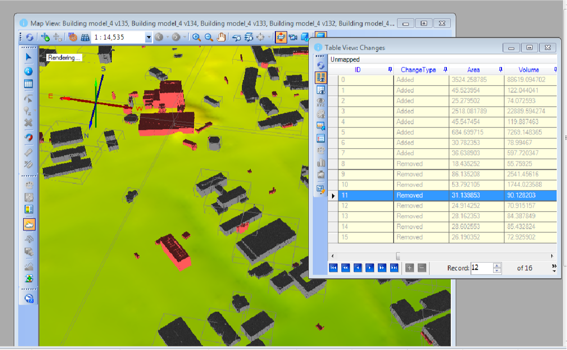
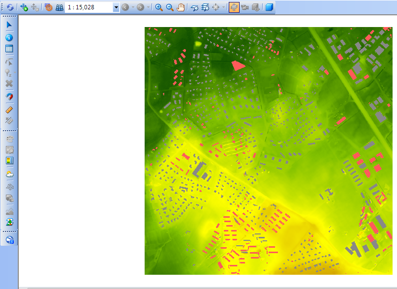
Modeled urban area with detected changes highlighted in red, two images for each of the three sites we’ve worked with before (two in Tallinn and one in Kharkiv). All these images come straight from the interface of my own modeling software, i.e. City Change Management.
Lasnamäe site
Lasnamäe site
Mustamäe site
Mustamäe site
Kharkiv site
Kharkiv site
4. Scoring & Final Table
4. Scoring & Final Table
In this third concluding phase, we take a close look at the processed datasets, evaluating them pair by pair with the trained similarity model . To keep things clear and ensure that we can compare class pairs effectively, we stick to mean similarity values that are representative of the broader statistical analysis from the study . This method helps us create final tables that offer a neat and understandable summary of the relationships between classes, complete with qualitative labels that highlight the thresholds set during the research
Summary scores that appear computed previously from resultsRaw
Detailed statistics, distinct from a final table
Final results—scores from referenceScores, with standard comparing interpretations
CITE THIS NOTEBOOK
CITE THIS NOTEBOOK
Neural networks reveal LiDAR-measured urban change and reconstruction patterns in war-affected Ukraine
by Sergiy Kostrikov
Wolfram Community, STAFF PICKS, September 29, 2025
https://community.wolfram.com/groups/-/m/t/3553061
by Sergiy Kostrikov
Wolfram Community, STAFF PICKS, September 29, 2025
https://community.wolfram.com/groups/-/m/t/3553061