ConchoidSurface::usage="The definition of a conchoid surface is:[u, v] = r[u, v] ± k , P is the pole, k distance and r[u, v] the base surface.In this notebook we will obtain the conchoid surface of the two-leaf hyperboloid: 2
r
c
r[u,v]-P
r[u,v]-P
-1+
Cos[v], 32
u
-1+
Sin[v], 4 u with the distance k = 1.5 and as pole P the {0, 0, 1}.Reference: Peternell, M. et al.Conchoid surfaces of rational ruled surfaces. Vienna University of Technology; Personal. ";2
u
Graph:
In[]:=
SwatchLegend[{Orange,Blue,Yellow},{"Positive conchoid surface","Negative conchoid surface","Base surface"}]Showr[u_,v_]:=2;r2[u_,v_]:=r[u,v]-k;{ParametricPlot3D[r1[u,v],{u,-5,5},{v,0,2π},PerformanceGoal"Quality",PlotStyle{Opacity[0.8],Orange},PlotPoints60],ParametricPlot3D[r2[u,v],{u,-5,5},{v,0,2π},PerformanceGoal"Quality",PlotStyle{Opacity[0.3],Blue},PlotPoints60],ParametricPlot3D[r[u,v],{u,-5,5},{v,0,2π},MeshFalse,PlotPoints60,PlotStyle->{Yellow,Opacity[0.8]}]},AxesLabel->(Style[#,15,Blue]&/@{"X","Y","Z"}),AxesOrigin{0,0,0},AxesTrue,BoxedFalse,BoxRatiosAutomatic,PlotLabelStyle[Framed["Conchoid surface of a two-leaf hyperboloid"],16,Blue,BackgroundYellow],PlotRange6,ViewPoint{-4,6,5.},ImageSize700
-1+
Cos[v],32
u
-1+
Sin[v],4u;k=1.5;P={0,0,1};r1[u_,v_]:=r[u,v]+k2
u
r[u,v]-P
Norm[r[u,v]-P]
r[u,v]-P
Norm[r[u,v]-P]
Out[]=


Out[]=

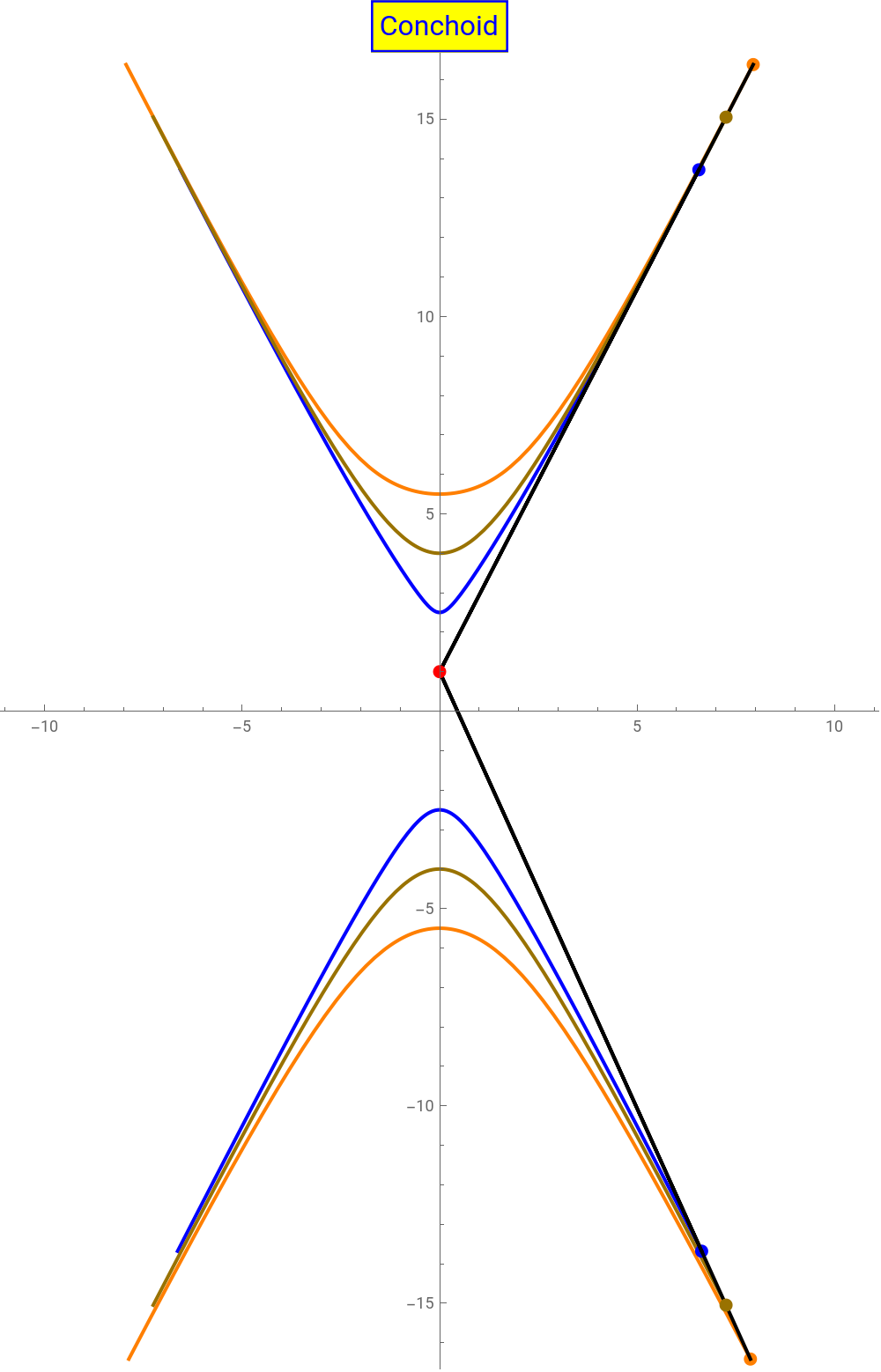
Explanation in 2D:
In[]:=
SwatchLegend[{Orange,Blue,DarkYellow,Red,Black},{"Positive Conchoid","Negative Conchoid","Original function","Pole","Generatrix line"}]Manipulatef[t_]:=2Sinh[t];g[t_]:=4Cosh[t];[t_]:=-4Cosh[t];=0;=1;k=1.5;[t_]:=f[t]++,g[t]++;[t_]:=f[t]-+,g[t]-+;[t_]:=f[t]++,[t]++;[t_]:=f[t]-+,[t]-+;Show[{ParametricPlot[[t],{t,-2,t1},PlotStyle{Orange,Thick},PerformanceGoal->"Quality"],ParametricPlot[[t],{t,-2,t1},PlotStyle{Blue,Thick},PerformanceGoal->"Quality"],ParametricPlot[[t],{t,-2,t1},PlotStyle{Orange,Thick},PerformanceGoal->"Quality"],ParametricPlot[[t],{t,-2,t1},PlotStyle{Blue,Thick},PerformanceGoal->"Quality"],ParametricPlot[{f[t],g[t]},{t,-2,2},PlotStyle{DarkYellow,Thick}],ParametricPlot[{f[t],[t]},{t,-2,2},PlotStyle{DarkYellow,Thick}],Graphics[{Orange,PointSize[0.015],Point[[t1]]}],Graphics[{Orange,PointSize[0.015],Point[[t1]]}],Graphics[{Blue,PointSize[0.015],Point[[t1]]}],Graphics[{Blue,PointSize[0.015],Point[[t1]]}],Graphics[{Black,Thick,Line[{[t1],{,},[t1]}]}],Graphics[{Black,Thick,Line[{[t1],{,},[t1]}]}],Graphics[{Red,PointSize[0.015],Point[{,}]}],Graphics[{DarkYellow,PointSize[0.015],Point[{f[t1],g[t1]}]}],Graphics[{DarkYellow,PointSize[0.015],Point[{f[t1],[t1]}]}]},AxesTrue,AxesOrigin{0,0},AspectRatioAutomatic,ImageSize500,PlotRange{{-10,10},{-15,15}},PlotLabelStyle[Framed["Conchoid"],16,Blue,BackgroundYellow]],{{t1,-2+0.00002,"Value (t1)"},-2+0.00001,2,0.00001},ControlPlacement->Top
g
1
x
0
y
0
ζ
+
k(f[t]-)
x
0
2
(f[t]-)
x
0
2
(g[t]-)
y
0
k(g[t]-)
y
0
2
(f[t]-)
x
0
2
(g[t]-)
y
0
ζ
-
k(f[t]-)
x
0
2
(f[t]-)
x
0
2
(g[t]-)
y
0
k(g[t]-)
y
0
2
(f[t]-)
x
0
2
(g[t]-)
y
0
ζ
1
+
k(f[t]-)
x
0
2
(f[t]-)
x
0
2
([t]-)
g
1
y
0
g
1
k([t]-)
g
1
y
0
2
(f[t]-)
x
0
2
([t]-)
g
1
y
0
ζ
1
-
k(f[t]-)
x
0
2
(f[t]-)
x
0
2
([t]-)
g
1
y
0
g
1
k([t]-)
g
1
y
0
2
(f[t]-)
x
0
2
([t]-)
g
1
y
0
ζ
+
ζ
-
ζ
1
+
ζ
1
-
g
1
ζ
+
ζ
1
+
ζ
-
ζ
1
-
ζ
-
x
0
y
0
ζ
+
ζ
1
-
x
0
y
0
ζ
1
+
x
0
y
0
g
1
Out[]=


Out[]=