2. Writing a BrinkmanPDEComponent
2. Writing a BrinkmanPDEComponent
BrinkmanPDEComponent yields a porous media flow PDE term with variables vars and parameters pars.
[vars,pars]
Definition
Definition
The BrinkmanPDEComponent[vars,pars] function provides the symbolic structure of the Brinkman’s equation for porous media flow. This function can take one of two sets of parameters:
1. Dynamic Viscosity, Porosity, and Permeability, or
2. Reynolds Number and Darcy Number
The function is defined as follows:
1. Dynamic Viscosity, Porosity, and Permeability, or
2. Reynolds Number and Darcy Number
The function is defined as follows:
In[]:=
Details
Details
◼
BrinkmanPDEComponent models the flow of viscous fluids through porous media under applied constraints.
◼
BrinkmanPDEComponent returns a sum of differential operators to be used as a part of partial differential equations:
BrinkmanPDEComponent[vars,...]〈boundarycondition〉
◼
BrinkmanPDEComponent creates PDE components for stationary parametric analysis.
◼
BrinkmanPDEComponent models fluid flow phenomena with velocities , and in units of [] as dependent variables, ∈ as independent variables in units of [].
u
v
w
m/s
x
i
n
m
◼
BrinkmanPDEComponent creates PDE components in two and three space dimensions
◼
Stationary variables are .
vars
vars={{u[,…,],v[,…,],…,p[,…,]},{,…,}}
x
1
x
n
x
1
x
n
x
1
x
n
x
1
x
n
◼
BrinkmanPDEComponent creates a system of equations with the vector-valued Brinkman’s momentum equation combined with the continuity equation.
◼
The equation of the model BrinkmanPDEComponent with dynamic viscosity μ [s Pa], porosity ϕ, and permeability κ is based on the Brinkman’s momentum equation and the continuity equation:
[]
2
m
μ κ μ ϕ | = | 0 |
∇·V | = | 0 |
◼
The Reynolds number is defined as ℛℯ = ρL/μ, where [] is a characteristic length and the flow velocity.
ℛℯ
U
L
m
U
◼
The Darcy number is defined as , where [] is a characteristic length, κ is the permeability, and ϕ is the porosity.
=κ
2
ϕL
L
m
[]
2
m
◼
The following parameters pars can be given:
parameter | default | symbol | |
"DynamicViscosity" | - | μ sPa | |
"Porosity" | - | ϕ | |
"Permeability" | - | κ [ 2 m | |
"ReynoldsNumber" | - | ℛℯ | |
"DarcyNumber" | - | ,Darcynumber |
◼
Dimensionless form of the Brinkman’s equations can be obtained by making the substitutions =V/ϕU, =p/ρ, and =x/L:
*
V
*
p
2
U
*
x
1 ℛℯ 1 ℛℯ | =0 |
∇·V | =0 |
◼
Instead of material parameters, a Reynolds number and a Darcy number can be specified.
ℛℯ
◼
BrinkmanPDEComponent uses units. The geometry has to be in the same units as the PDE.
"SIBase"
Examples
Examples
Basic Examples
Basic Examples
Define flow PDE through a porous medium:
In[]:=
BrinkmanPDEComponent[{{u[x,y],v[x,y],p[x,y]},{x,y}},<|"DynamicViscosity"->μ,"Porosity"->ϕ,"Permeability"->κ|>]//MatrixForm
Out[]//MatrixForm=
10000u[x,y]+ ∇ {x,y} ∇ {x,y} (1,0) p |
10000v[x,y]+ ∇ {x,y} ∇ {x,y} (0,1) p |
(0,1) v (1,0) u |
Define stationary flow PDE model through porous medium with Reynolds number of 10 and Darcy number of :
-4
10
In[]:=
BrinkmanPDEComponent[{{u[x,y],v[x,y],p[x,y]},{x,y}},<|"ReynoldsNumber"->10,"DarcyNumber"->|>]//MatrixForm
-4
10
Out[]//MatrixForm=
1000u[x,y]+ ∇ {x,y} 1 10 ∇ {x,y} (1,0) p |
1000v[x,y]+ ∇ {x,y} 1 10 ∇ {x,y} (0,1) p |
(0,1) v (1,0) u |
Scope
Scope
Specify a flow PDE through porous medium with dynamic viscosity of , porosity of 0.4, and permeability of :
-3
10
-7
10
In[]:=
BrinkmanPDEComponent[{{u[x,y],v[x,y],p[x,y]},{x,y}},<|"DynamicViscosity"->,"Porosity"->0.4,"Permeability"->|>]//MatrixForm
-3
10
-7
10
Out[]//MatrixForm=
10000u[x,y]+ ∇ {x,y} ∇ {x,y} (1,0) p |
10000v[x,y]+ ∇ {x,y} ∇ {x,y} (0,1) p |
(0,1) v (1,0) u |
Activate a flow PDE through porous medium with Reynolds number of 0.5 and Darcy number of :
-2
10
In[]:=
Activate[BrinkmanPDEComponent[{{u[x,y],v[x,y],p[x,y]},{x,y}},<|"ReynoldsNumber"->0.5,"DarcyNumber"->|>]]
-2
10
Out[]=
200.u[x,y]-2.[x,y]+[x,y]-2.[x,y],200.v[x,y]+[x,y]-2.[x,y]-2.[x,y],[x,y]+[x,y]
(0,2)
u
(1,0)
p
(2,0)
u
(0,1)
p
(0,2)
v
(2,0)
v
(0,1)
v
(1,0)
u
Specify a symbolic stationary flow PDE through porous medium in two dimensions with dynamic viscosity μ, porosity ϕ, and permeability κ:
In[]:=
BrinkmanPDEComponent[{{u[x,y],v[x,y],p[x,y]},{x,y}},<|"DynamicViscosity"->μ,"Porosity"->ϕ,"Permeability"->κ|>]
Out[]=
10000u[x,y]+·(-0.0025u[x,y])+[x,y],10000v[x,y]+·(-0.0025v[x,y])+[x,y],[x,y]+[x,y]
∇
{x,y}
∇
{x,y}
(1,0)
p
∇
{x,y}
∇
{x,y}
(0,1)
p
(0,1)
v
(1,0)
u
Specify a symbolic stationary flow PDE through porous medium in three dimensions with dynamic viscosity μ, porosity ϕ, and permeability κ:
In[]:=
BrinkmanPDEComponent[{{u[x,y,z],v[x,y,z],w[x,y,z],p[x,y,z]},{x,y,z}},<|"DynamicViscosity"->μ,"Porosity"->ϕ,"Permeability"->κ|>]
Out[]=
10000u[x,y,z]+·(-0.0025u[x,y,z])+[x,y,z],10000v[x,y,z]+·(-0.0025v[x,y,z])+[x,y,z],10000w[x,y,z]+·(-0.0025w[x,y,z])+[x,y,z],[x,y,z]+[x,y,z]+[x,y,z]
∇
{x,y,z}
∇
{x,y,z}
(1,0,0)
p
∇
{x,y,z}
∇
{x,y,z}
(0,1,0)
p
∇
{x,y,z}
∇
{x,y,z}
(0,0,1)
p
(0,0,1)
w
(0,1,0)
v
(1,0,0)
u
Applications
Applications
Stationary Analysis
Stationary Analysis
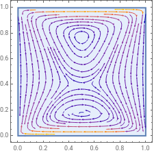
Solve for the velocity and pressure in a porous cavity with antiparallel flow and a source term:
In[]:=
source={If[0.4<=x<=0.6&&0.4<=y<=0.6,100,0],0,0};{uVel,vVel,pressure}=NDSolveValue[{BrinkmanPDEComponent[{{u[x,y],v[x,y],p[x,y]},{x,y}},<|"ReynoldsNumber"->0.5,"DarcyNumber"->|>]+source=={0,0,0},DirichletCondition[{u[x,y]==1,v[x,y]==0},y==1],DirichletCondition[{u[x,y]==0,v[x,y]==0},0<y<1],DirichletCondition[{u[x,y]==-1,v[x,y]==0},y==0],DirichletCondition[p[x,y]==0,x==0&&y==0]},{u[x,y],v[x,y],p[x,y]},{x,y}∈Rectangle[{0,0},{1,1}],Method->{"FiniteElement","InterpolationOrder"->{u->2,v->2,p->1}}];
-2
10
Visualize the velocity of the fluid:
In[]:=
StreamPlot[{uVel,vVel},{x,y}∈Rectangle[{0,0},{1,1}]]
Out[]=