Physics-Principles with Applications Douglas C. Giancoli 7th Edition Publisher Pearson ISBN-13 978-0-321-62592-2 Chapter 5-CIRCULAR MOTION
PeterBurbery
I really like the textbook Giancoli Physics. Mathematica has many powerful functions for manipulating physical quantities that I use to practice problem solving with physics.
*5-4 Nonuniform Circular Motion
*5-4 Nonuniform Circular Motion
In[]:=
25*(II) A car at the Indianapolis 500 accelerates uniformly from the pit area, going from rest to 270 km/h in a semicircular arc with a radius of 220 m. Determine the tangential and radial acceleration of the car when it is halfway through the arc, assuming constant tangential acceleration. If the curve were flat, what coefficient of static friction would be necessary between the tires and the road to provide this acceleration with no slipping or skidding?
25*(II) A car at the Indianapolis 500 accelerates uniformly from the pit area, going from rest to 270 km/h in a semicircular arc with a radius of 220 m. Determine the tangential and radial acceleration of the car when it is halfway through the arc, assuming constant tangential acceleration. If the curve were flat, what coefficient of static friction would be necessary between the tires and the road to provide this acceleration with no slipping or skidding?
I use all capital letters for names of equations.
In[]:=
FIRSTKINEMATICSEQUATION===+2()()
2
v
R
2
v
P
a
tan
PR
Out[]=
2
v
R
PR
a
tan
2
v
P
In[]:=
$rules={}
Out[]=
{}
In[]:=
$rules//=Flatten[Append[Solve[FIRSTKINEMATICSEQUATION,]][#]]&
a
tan
Out[]=
-+
a
tan
2
v
P
2
PR
2
v
R
2
PR
In[]:=
SECONDKINEMATICSEQUATION===+2()()
2
v
Q
2
v
P
a
tan
PQ
Out[]=
2
v
Q
PQ
a
tan
2
v
P
In[]:=
$rules//=Flatten[Append[#][Refine[Solve[SECONDKINEMATICSEQUATION,,],{>0∧>0∧>0}]//.#]]&
v
Q
≥0
a
tan
v
P
PQ
Out[]=
+2-+,-+
v
Q
2
v
P
PQ
2
v
P
2
PR
2
v
R
2
PR
a
tan
2
v
P
2
PR
2
v
R
2
PR
In[]:=
CENTRIPETALACCELERATION=-==0
a
c
2
v
Q
r
Out[]=
a
c
2
v
Q
r
In[]:=
$rules//=Flatten[Append[#][Solve[CENTRIPETALACCELERATION,]//.#]]&
a
c
Out[]=
+2-+,+2-+,-+
a
c
2
v
P
PQ
2
v
P
2
PR
2
v
R
2
PR
r
v
Q
2
v
P
PQ
2
v
P
2
PR
2
v
R
2
PR
a
tan
2
v
P
2
PR
2
v
R
2
PR
In[]:=
NONUNIFORMCIRCULARMOTIONEQUATION===+
a
2
a
c
2
a
tan
Out[]=
a
2
a
c
2
a
tan
In[]:=
$rules//=Flatten[Append[#][Solve[NONUNIFORMCIRCULARMOTIONEQUATION,]//.#]]&
a
Out[]=
++2-+,+2-+,+2-+,-+
a
2
-+
2
v
P
2
PR
2
v
R
2
PR
2
2
v
P
PQ
2
v
P
2
PR
2
v
R
2
PR
2
r
a
c
2
v
P
PQ
2
v
P
2
PR
2
v
R
2
PR
r
v
Q
2
v
P
PQ
2
v
P
2
PR
2
v
R
2
PR
a
tan
2
v
P
2
PR
2
v
R
2
PR
In[]:=
FRICTIONEQUATION=()()-==0;
m
g
μ
m
a
In[]:=
$rules//=Flatten[Append[#][Solve[FRICTIONEQUATION,]//.#]]&
μ
Out[]=
++2-+,++2-+,+2-+,+2-+,-+
μ
2
-+
2
v
P
2
PR
2
v
R
2
PR
2
2
v
P
PQ
2
v
P
2
PR
2
v
R
2
PR
2
r
g
a
2
-+
2
v
P
2
PR
2
v
R
2
PR
2
2
v
P
PQ
2
v
P
2
PR
2
v
R
2
PR
2
r
a
c
2
v
P
PQ
2
v
P
2
PR
2
v
R
2
PR
r
v
Q
2
v
P
PQ
2
v
P
2
PR
2
v
R
2
PR
a
tan
2
v
P
2
PR
2
v
R
2
PR
numerical values
numerical values
Substitute the values given:
In[]:=
$keys={,,,,,};
r
v
P
v
R
PQ
PR
g
In[]:=
$values$with$standard$gravity=,,,FullSimplifyRegionMeasureRegion,FullSimplifyRegionMeasureRegion,;

In[]:=
$values$with$current$gravitational$field$strength$magnitude=,,,FullSimplifyRegionMeasureRegion,FullSimplifyRegionMeasureRegion,GeogravityModelData["Magnitude"];
In[]:=
$rules$with$standard$gravity=AssociationThread[$keys->$values$with$standard$gravity]
Out[]=
,,,,,
r
v
P
v
R
PQ
PR
g
In[]:=
$rules$with$current$gravitational$field$strength$magnitude=AssociationThread[$keys->$values$with$current$gravitational$field$strength$magnitude]
Out[]=
,,,,,
r
v
P
v
R
PQ
PR
g
Compute the value of the quantities with standard gravity:
In[]:=
$rules//.$rules$with$standard$gravity/.q_?QuantityQ->UnitConvert[q,"SIBase"]
Out[]=
,,,,
μ
125+
3321506250000
121
3321506250000
121
2
π
15886773
a
a
c
v
Q
a
tan
Compare the numerical result with standard gravity to the numerical result with local gravity (the only value that's different is μ):
In[]:=
$rules//.$rules$with$standard$gravity/.q_?QuantityQ->UnitConvert[q,"SIBase"]//N
Out[]=
1.36806,,,,
μ
a
a
c
v
Q
a
tan
In[]:=
$rules//.$rules$with$current$gravitational$field$strength$magnitude/.q_?QuantityQ->UnitConvert[q,"SIBase"]//N
Out[]=
1.36906,,,,
μ
a
a
c
v
Q
a
tan
I will round the centripetal acceleration and tangential acceleration to compare my answer with the books's answer.
In[]:=
AssociationThread[{,,}->MapThread[Round[#1,#2]&,{Lookup[$rules//.$rules$with$standard$gravity/.q_?QuantityQ->UnitConvert[q,"SIBase"]//N,{,,}],{0.1,1,0.1}}]]
a
tan
a
c
μ
a
tan
a
c
μ
Out[]=
,,1.4
a
tan
a
c
μ
The textbook lists the answer as =4.1 m/, =13 m/, and 1.4 for the coefficient of static friction needed.
a
tan
2
s
a
rad
2
s
the circle
the circle
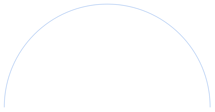
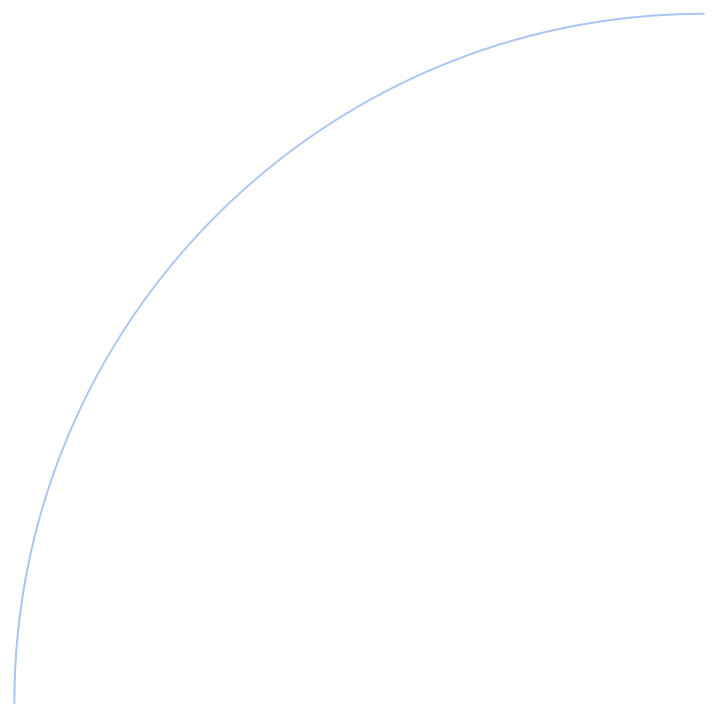
Here's are some pictures for the exercise:
In[]:=
Region[Circle[{0,0},220,{0Degree,180Degree}]]
Out[]=
In[]:=
Region[Circle[{0,0},220,{90Degree,180Degree}]]
Out[]=
Here's a graphic I made:
Here is a picture with the points labeled. Click on the points to see their names. The name of an arc of a circle is the name of the starting and ending points. For example an arc could be named PQ if it went from point P to point Q. The length of the arc is denoted by PQ in this case. Below this, there is a graphic that displays a tooltip with the name of a point when you hover over it instead of opening up a popup window.