The Geneva mechanism is a type of gear train that allows for precise, intermittent motion. It is composed of a driving wheel with a pin and a driven wheel with slots. The pin enters the slots of the driven wheel and rotates it step-by-step. The driving wheel also has an elevated half-circle, which locks the driven wheel in position between the steps. Geneva mechanisms are used in a variety of applications, including: film cameras, watches, music boxes, robotics, and medical devices.
In this notebook, the NDSolve, If, and Manipulate commands are used to analyze and simulate four-, five-, six-, and seven-slot Geneva mechanisms. The NDSolve command is used to solve the differential equations that describe the motion of the Geneva mechanism. The If command is used to control the flow of the simulation, and the Manipulate command is used to create interactive controls that allow the user to change the parameters of the simulation. The simulation can be used to design and optimize Geneva mechanisms for specific applications.
In this notebook, the NDSolve, If, and Manipulate commands are used to analyze and simulate four-, five-, six-, and seven-slot Geneva mechanisms. The NDSolve command is used to solve the differential equations that describe the motion of the Geneva mechanism. The If command is used to control the flow of the simulation, and the Manipulate command is used to create interactive controls that allow the user to change the parameters of the simulation. The simulation can be used to design and optimize Geneva mechanisms for specific applications.
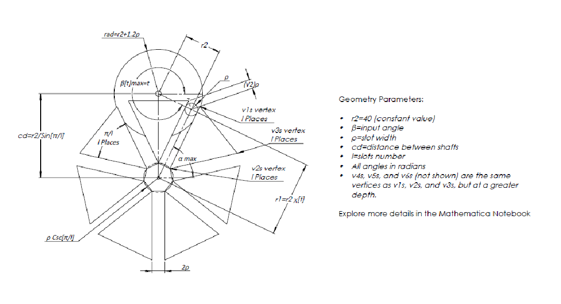
Geneva Mechanism Schematic View
Geneva Mechanism Schematic View
Figure1.GeometricParametersoftheanalyzedGenevaMechanismwithsevenslotsNomenclaturer1:distancemeasurementbetweenthelowerdrivenshaftandthepincenterTheequationforr1isr2X[t],wherer2isanotherdistancemeasurementandχ[t]isadimensionlesstermα:Anglebetweenthehorizontalandradiusr1r2:Distancebetweentheupperdrivingshaftandpincenter(40inthiscase)β:Anglebetweenthehorizontalandradiusr2
Kinematic Analysis
Kinematic Analysis
Displacement Equations
Displacement Equations
In[]:=
Clear[r2,cd,α,β,t];(*r1=r2χ[t]*)ξ=r2χ[t]Cos[α[t]]-r2Cos[β[t]]==0;(*Equationfordisplacementsalongxaxis*)ψ=r2χ[t]Sin[α[t]]-r2Sin[β[t]]==cd;(*Equationfordisplacementsalongzaxis*)
Velocity Equations
Velocity Equations
In[]:=
Dt[{ξ,ψ},t,Constants->{cd,r2}](*Derivingthedisplacementequations,whicharealsodifferentialequationsthatdescribevelocity*)
Out[]=
{-r2Sin[α[t]]χ[t][t]+r2Sin[β[t]][t]+r2Cos[α[t]][t]0,r2Cos[α[t]]χ[t][t]-r2Cos[β[t]][t]+r2Sin[α[t]][t]0}
′
α
′
β
′
χ
′
α
′
β
′
χ
Solving the System of Differential Equations
Solving the System of Differential Equations
Entry angle β is a known input equal to time, β [t] = t, and the input angular velocity is taken as = 1 rad/s.Equations from Velocity Equations section are rewritten so that they can be solved with NDSolve.The initial values, , are taken from analysis of Figure 1.
′
β
α==,χ==Cot
8π
7
9π
14
8π
7
π
7
In[]:=
r2=40;s=NDSolve-r2Sin[α[t]]χ[t][t]+r2Sin[t]+r2Cos[α[t]][t]0,r2Cos[α[t]]χ[t][t]-r2Cos[t]+r2Sin[α[t]][t]0,α==,χ==Cot,{α,χ},t,,
′
α
′
χ
′
α
′
χ
8π
7
9π
14
8π
7
π
7
8π
7
13π
7
Out[]=
αInterpolatingFunction,χInterpolatingFunction


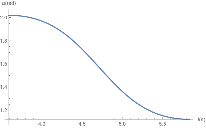
Displacement plot
Displacement plot
In[]:=
PlotEvaluate[{α[t]}/.s],t,,,FrameFalse,AxesLabel{"t(s)","α(rad)"},PlotRangeAll(*Plotstheangulardisplacementofα*)
8π
7
13π
7
Out[]=
Manipulate
Manipulate
In[]:=
Out[]=


CITE THIS NOTEBOOK
CITE THIS NOTEBOOK
Geneva mechanism simulation
by David Balandra
Wolfram Community, STAFF PICKS, September 18, 2023
https://community.wolfram.com/groups/-/m/t/3014615
by David Balandra
Wolfram Community, STAFF PICKS, September 18, 2023
https://community.wolfram.com/groups/-/m/t/3014615