The Prisoner’s Dilemma is a matrix game that represents the tension between cooperation and competition. In a one-off game, without knowing the opponent’s action, players benefit most from playing the Nash equilibrium. However, when this game is repeated multiple times, each player learns from the opponent and can employ strategies that will benefit them most in the long term. Axelrod’s tournaments tested approximately 100 strategies; yet, there are infinitely many possible strategies a player can employ. This project aims to simulate the repeated prisoner’s dilemma between 196900 strategies generated from BooleanFunction. The analysis of these tournaments provides some insight into properties that tend to make certain strategies more successful than others and can be extended to the study of other matrix games.
Introduction
Introduction
The Prisoner’s Dilemma
The Prisoner’s Dilemma
Matrix games are models of decision-making scenario in which all players act simultaneously without knowing the opponent’s move. Its payoff matrix represents the potential outcomes of combinations of moves made by all parties in a game. The simplest version of these games involve two players, each with two possible actions to choose from.
The Prisoner’s Dilemma is a classic example of such a matrix game used to represent the tension between an individual and the collective’s benefit. A player can choose to either cooperate or defect in any round, knowing the consequences for all players in the game. An example of the matrix game between two players (which we will be utilizing throughout this simulation) is below.
In[]:=
game=MatrixGame{{{-5,-5},{0,-10}},{{-10,0},{-1,-1}}},;
In[]:=
game["Dataset"]
Out[]=
|

In[]:=
MatrixGamePlot[game]
Out[]=
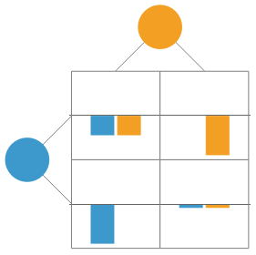


With both players having perfect information, we can find the Nash equilibrium of this matrix game. The Nash equilibrium is the state in a matrix game in which no player will benefit or lose more by changing their strategy, given that all other players’ strategies remain constant. With the prisoner’s dilemma analogy, a player will want to minimize the number of years they spend in prison, so they would want to get a number closest to zero. In Wolfram Language, we can employ FindMatrixGameStrategies to find this equilibrium.
In[]:=
FindMatrixGameStrategies[game]
Out[]=
{{{1,0},{1,0}}}
In this game, the Nash Equilibrium lies at row 1 column 1, which is when both players choose to defect. Thus, in a one-round game of Prisoner’s Dilemma, both players are better off choosing to defect when they don’t know the other player’s move, even if both players earn a better payoff when they both choose to cooperate; however, choosing to cooperate would put them at risk of getting -10 when the other chooses to defect.
Repeated Prisoner’s Dilemma
Repeated Prisoner’s Dilemma
Such a game isn’t confined to the bounds of an n x n matrix that one chooses to play. The Prisoner’s Dilemma models daily interactions in economics, politics, diplomacy, etc. These actors do not only have these kinds of interactions once but multiple times, learning how other players react in different scenarios. So, naturally, one question arises: what strategy should one employ when the prisoner’s dilemma is played for multiple rounds?
Robert Axelrod, a political science professor at the University of Michigan, modeled this scenario by asking several game theorists to submit a strategy in a round robin. One famous strategy is the grim trigger, where a player cooperates until the opponent defects. However, the strategy that rose atop was the Tit for Tat in which a player chooses to cooperate in the first round and, for all future rounds, the player chooses whatever the opponent chose in the previous round. From this tournament, he identified four properties that tend to make a strategy successful: “avoidance of unnecessary conflict by cooperating as long as the other player does, provocability in the face of an uncalled-for defection by the other, forgiveness after responding to a provocation, and clarity of behavior so that the other player can recognize and adapt to your pattern of action” (Axelrod 1984).
In these tournaments, only a limited number of strategies were tested. Here, we aim to simulate all possible strategies a player can employ, generated from BooleanFunction, over the course of a simulation of the repeated prisoner’s dilemma.
An Example Simulation
An Example Simulation
A Note about MatrixGamePayoff
A Note about MatrixGamePayoff
Throughout this essay, I’ll be utilizing a modified version of MatrixGamePayoff as BooleanFunction outputs True or False (which we Boole to 1 or 0), which is not an acceptable input for MatrixGamePayoff. This modification will prevent us from repeatedly changing data types throughout the simulations.
In[]:=
matrixGamePayoffMod[game_,player1_Integer,player2_Integer]:=Module[{play1,play2}, If[player1==1, play1={1,0},play1={0,1}]; If[player2==1, play2={1,0},play2={0,1}]; MatrixGamePayoff[game,{play1,play2}]]
An Example Simulation between Rules 0 and 1
An Example Simulation between Rules 0 and 1
We’ll first walk through an example in a game of four rounds in which player 1 uses Boolean rule 0 against player 2 using Boolean rule 1 in a Prisoner’s Dilemma, taking into account the other player’s previous two moves. First, we initialize the conditions.
rulep1 and rulep2 set the rule for each player to be the BooleanFunction 0 and 1, respectively. The 2 in the Boolean function specifies the number of moves a player takes into consideration. In this case, it’s the two previous moves of the other player.
In[]:=
rulep1=BooleanFunction[0,2];rulep2=BooleanFunction[1,2];
Sets the first two moves of each player to Defect (which we will see as True or 1; Cooperate will be False or 0)
In[]:=
move1p1=1;move2p1=1;move1p2=1;move2p2=1;
Sets the score of each player to 0, creates a list to track score, and another list to track the moves employed by each player, including the first two. These lists will become useful when we want to see the change over time or any relevant statistics.
In[]:=
scorep1=0;scorep2=0;scorelistp1=List[];scorelistp2=List[];movelistp1={1,1};movelistp2={1,1};
Calculate the payoff for the first two inputted moves and add them to their score.
Move 1
In[]:=
payoffmove1=matrixGamePayoffMod[game,move1p1,move1p2]
Out[]=
{-5,-5}
In[]:=
scorep1+=payoffmove1[[1]]
Out[]=
-5
In[]:=
AppendTo[scorelistp1,scorep1]
Out[]=
{-5}
In[]:=
scorep2+=payoffmove1[[2]]
Out[]=
-5
In[]:=
AppendTo[scorelistp2,scorep2]
Out[]=
{-5}
Move 2
In[]:=
payoffmove2=matrixGamePayoffMod[game,move2p1,move2p2]
Out[]=
{-5,-5}
In[]:=
scorep1+=payoffmove2[[1]];AppendTo[scorelistp1,scorep1]
Out[]=
{-5,-10}
In[]:=
scorep2+=payoffmove2[[2]];AppendTo[scorelistp2,scorep2]
Out[]=
{-5,-10}
Now that we’ve initialized all necessary conditions, we look at the third move each player will make according to their BooleanFunction and the other player’s two previous moves.
In[]:=
move3p1boole=rulep1[move1p2,move2p2]
Out[]=
False
In[]:=
move3p2boole=rulep2[move1p1,move2p1]
Out[]=
False
As matrixGamePayoffMod takes in 0 and 1, we want to store our variable in such a way instead using Boole. It’s also easier for data storage and handling in general.
In[]:=
move3p1=Boole[move3p1boole]
Out[]=
0
In[]:=
move3p2=Boole[move3p1boole]
Out[]=
0
Both players output 0, which means they choose to cooperate. We add both of these moves to their movelist.
In[]:=
AppendTo[movelistp1,move3p1]
Out[]=
{1,1,0}
In[]:=
AppendTo[movelistp2,move3p2]
Out[]=
{1,1,0}
Calculate each of their payoffs and add them to their scores and lists.
In[]:=
payoffmove3=matrixGamePayoffMod[game,move3p1,move3p2]
Out[]=
{-1,-1}
In[]:=
scorep1+=payoffmove3[[1]];AppendTo[scorelistp1,scorep1]
Out[]=
{-5,-10,-11}
In[]:=
scorep2+=payoffmove3[[2]];AppendTo[scorelistp2,scorep2]
Out[]=
{-5,-10,-11}
Moving on to round 4, we again start by calculating their moves.
In[]:=
move4p1=Boole[rulep1[move2p2,move3p2]]
Out[]=
0
In[]:=
move4p2=Boole[rulep2[move2p1,move3p1]]
Out[]=
0
Add the moves to their respective lists
In[]:=
AppendTo[movelistp1,move4p1];AppendTo[movelistp2,move4p2];
Calculate their payoffs and add them to their scores and lists
In[]:=
payoffmove4=matrixGamePayoffMod[game,move4p1,move4p2]
Out[]=
{-1,-1}
In[]:=
scorep1+=payoffmove4[[1]];AppendTo[scorelistp1,scorep1]
Out[]=
{-5,-10,-11,-12}
We’ve successfully gone through four rounds of the Prisoner’s Dilemma using these two rules. We now visualize their cumulative score over time.
As the lines fully intersect, both player perform equally throughout these four rounds. However, this does not mean that they will tie as the payoffs may change in future rounds not simulated above.
Main Simulation
Main Simulation
Strategies
Strategies
One important question that comes with this simulation is what strategies can a player employ. To tackle this issue, there are three main factors.
Firstly, we consider what moves the player takes into consideration. We split them into three categories:
◼
“Join” : The player considers both their own moves and the other’s by joining the list end-to-end. From player1’s perspective, the input list would be {move1p1,...,movenp1,move1p2,...,movenp2}, and player 2’s would be {move1p2,...,movenp2,move1p1,...,movenp1}.
◼
“Riffle”: The player considers both their own moves and the other’s by riffling the lists together. Player 1’s input would look like {move1p1,move1p2,...,movenp1,movenp2}, and player 2’s would be {move1p2,move1p1,...,movenp2,movenp1}.
◼
“Only” : The player only considers the moves played by the other player. For example, from player 1’s perspective, the input into the BooleanFunction could be {move1p2,move2p2,...}.
Secondly, we must also consider how many previous rounds will a player take into consideration in the BooleanFunction. The higher the number of rounds considered, the more possible strategies there are. Let’s take a look at some examples:
◼
If a player uses “Only” and considers the 2 previous round, their input would have 2 entries, and they can choose from 2^2^2=16 rules
◼
If a player uses “Join” and considers only the most previous round, their input has 2 entries (one for each player), and they can choose from 2^2^2=16 rules
◼
If a player uses “Riffle” and considers 2 rounds, their input would have 4 entries (two for each player), and they can choose from 2^2^4=65536 rules
One other thing that needs to be considered is the initial moves a player can make before their strategy activates. This can be any permutation of 0s and 1s of as many round a player takes into consideration.
Ranking
Ranking
To be able to extract more data from a round robin tournament (or any multiple matchups between different strategies), we create a function that finds the rate each strategy win, lose, and tie, the rate of cooperation and defect, and the total score over all the rounds within a tournament.
statsRule takes the tabled results from booleanStrategy2PlayersAdapt as an argument. Instead of ranking by win rate, we rank the strategies by their total score to represent the total tradeoff a player would confront.
As an example output, we run the function over the round robin tournament we ran above between all the “Only” strategies that take in only one previous round.
Tournament
Tournament
Although there are infinitely many possible strategies that can be generated with the BooleanFunction, we are unable to test for all possibilities. Considering the amount of rounds a player in reality will consider, we will only examine “Only” with 4 previous rounds and “Join” and “Riffle” for 2 previous rounds. In fact, due to computational limitations, we can only consider strategies that take in 4 inputs into the BooleanFunction as having five inputs increases the rule possibility to 2^2^5 = 4294967296 (over 4 billion).
We create all the possible rules that we will examine. In the list below, we presume that their initial moves are cooperate. To change this initial condition, you can manipulate the last entry of the list.
There are 196900 strategies possible from this list (when the initial plays are all fixed to cooperate). Again, due to computational limitations, we cannot run a round robin with all rules. Thus, we must create a tournament between only some strategies from the list.
This tournament will consists of two stage. The first stage is split into 50 different pools where in each pool, 100 random strategies face off each other in a round robin. The top five from each of these pools move on to the second stage, competing in a round robin against the other 249 top-performing strategies.
testingPairs simulates one round robin in the semifinals. The function finds random sample of size 100 from the list and delete those entries from it. Then, it applies booleanStrategy2PlayersAdapt and statsRule to them, taking the top 5 scorers.
tournament competes the top 5 strategies from each of the rounds into a round robin.
Due to computational limitations, it’s more feasible to run these functions separately. The code to run all the function is below. Before running each tournament, make sure to rerun the alljoinriffleonly to restore every strategy in the list.
Results
Results
Initial Plays Fixed to Cooperate
Initial Plays Fixed to Cooperate
We fix the initial plays for all players to be cooperate and run the tournament using the strategies in allrifflejoinonly. After running the tournament four times, we receive the following data:
Due to the large memory requirements and evaluation time, the data from the simulations was saved in Wolfram Cloud and are hereby imported.
Plots
Plots
We now plot some of the data to find any correlation within or between any of the variables.
A Table Count of Different Strategy
In all three tournaments, most of the strategies that advanced to the final round are “Riffle” and “Join” with only around 10% of each tournament being “Only,” and even those that are in the finals rank very low in the tournament. This difference in counts illustrates that, starting with cooperation, “Riffle” and “Join” tend to do better. Additionally, if we inspect the actual data, we can see that all the “Riffle” and “Join” consider the 2 previous rounds and “Only” examines the 4 previous rounds, which means all of the strategies take in 4 arguments to the BooleanFunction. This could help us infer that when starting with cooperation, strategies that tend to do better take in more arguments to the BooleanFunction.
A Histogram of the Scores of Each Tournament
The score distribution for all three tournaments is approximately bimodal with a higher peak between -19000 to -17000 and a smaller peak between -47000 and -45000. These distinct peaks demonstrate that strategies which start with cooperation either score well or poorly, not really in between those extremes.
A Scatter Plot between the Rate of Cooperation and Score
In all three plots, there are 2 main clusters: one with a lower cooperation rate (0-0.5) and another with a higher cooperation rate (0.8-1.0). The cluster with a lower cooperation rate has a lower cumulative score while the cluster with a higher cooperation rate has a higher cumulative score. These groupings suggest that a player will score higher if their strategy involves more cooperation. However, within each cluster, there is a negative correlation between the data points, especially in the cluster that cooperates more. This trend indicates that strategies that tend to be more successful in that cluster has a wise balance between cooperating and defecting.
In[]:=
A Scatter Plot between Rate of the Cooperation and Wins
Similar to the rate of cooperation and score plots, these plots also display two distinct clusters. The lower cooperation rate cluster (0-0.5) has a higher win rate than the higher cooperation rate cluster (0.8-1.0), each having its own negative correlation. These clusters agree with overall inverse relationship between win rate and cooperation rate presented in all three plots.
Analysis
Analysis
For strategies that have cooperate as their initial plays, strategies that tend to score better have a higher cooperation rate while strategies that tend to win more defect more.
Initial Plays Fixed to Defect
Initial Plays Fixed to Defect
These are the lists used to run the tournament when all initial plays are defect.
Here, we run the tournament three times.
Due to the large memory requirements and evaluation time, the data from the simulations was saved in Wolfram Cloud and are hereby imported.
Plots
Plots
A Table Count of Different Strategy
The strategy count for initial plays being defect is similar to when they were cooperate. “Join” and “Only” are the majority of the strategies being employed while “Only” constitutes a minor portion of the whole. Other trends also remain consistent with those discussed earlier.
A Histogram of the Scores of Each Tournament
The histogram portrays a bimodal distribution with a higher peak -58000 and -55000 and a smaller peak -73000 to -70000. The relative score of these strategies when compared to the when initial plays were cooperate is a lot lower likely due to the fact that most strategies end up choosing to defect, which has a higher payoff risk.
A Scatter Plot Between the Rate of Cooperation and Score
Contrary to when the initial plays were all cooperate, the overall correlation between cooperate rate and score is negative. Thus, rather than indicating a two “separate” trends, these plots only show that a player tends to be more successful when they defect more.
A Scatter Plot Between the Rate of Cooperation and Wins
These scatter plots appear to have no overall correlation entirely, even within the ambiguous 2 clusters present in the three graphs. Thus, if the initial plays are defect, there is likely no relationship between the cooperation rate and win rate.
Analysis
Analysis
If every player in the game has their initial plays fixed at defect, strategies that has a lower cooperation rate tend to be more successful score-wise.
Initial Plays Randomized
Initial Plays Randomized
These are the lists used to run the tournament when all initial plays are randomized
We run the tournaments three times.
Due to the large memory requirements and evaluation time, the data from the simulations was saved in Wolfram Cloud and are hereby imported.
Plots
Plots
A Table Count of Different Strategy
The only strategies that pass on to the final round when the initial plays are randomized are only, which is quite surprising when we compare this to when initial plays were all cooperate or all defect. Most of these “Only” strategies take in 4 rounds of input to be considered; however, in finalsrandom3, the strategy that performed the best only took in one input. Although this may appear to be an anomaly, we are unable to come to this conclusion as out of the 196900 strategies, there are only 4 “Only” strategies that take in one round of input, which means they might not have been in any of the other tournaments we have simulated.
A Histogram of the Scores of Each Tournament
The score distribution when initial plays are randomized is unimodal with the peak lying between -53000 and -49000. This distribution, weakly looking similar to an F distribution (although here in a negative domain), illustrates that these strategies don’t tend to perform in the extremes like the previous sets we’ve looked at.
A Scatter Plot Between the Rate of Cooperation and Score
From these plots, we can see a moderately strong negative correlation between cooperation rate and score. This means that strategies that tend to score better has a lower cooperation rate.
A Scatter Plot between the Rate of Cooperation and Wins
Similar to the relation between cooperation and score, there is a relatively strong negative relationship between the cooperation and win rate. Thus, if we combine the two observations from these two plots, we can infer that the score and win rate has a positive relationship, unlike the relationship seen when initial plays are all fixed to cooperate.
Analysis
Analysis
From these simulations, we can partially infer that strategies that tend to see more success are those that only considers the opponent’s moves. Between this group of strategies, the ones that have a better score and a higher win rate are those that defect more.
Overall Analysis of the Repeated Prisoner’s Dilemma Simulation
Overall Analysis of the Repeated Prisoner’s Dilemma Simulation
From the three separate initial plays conditions, we gained very different insight into the rate of cooperation to the success of different strategies in repeated prisoner’s dilemma. In the case when initial plays are cooperate, the relative rate of cooperation of a strategy gives its own benefits: those that have a higher cooperation rate score better while those with a higher defect rate win more games. In the case when we fix initial plays to defect, a higher cooperation rate indicates worse performance in terms of score. Lastly, when the initial plays were randomized, there exists a relatively strong negative correlation between cooperation rate and both score and win rate.
These different findings for different initial play conditions show that the use of each strategy is highly dependent on the initial plays that a player employs before their strategy is activated. Thus, to come to a more conclusive statement, we must be able to test all these initial plays head-to-head. This modification would amount the number of total strategies to over one million possibilities.
Other Games
Other Games
booleanStrategy2PlayersAdapt can be easily adapted to be used with other matrix games simply by changing the initialization game matrix. After that, running the same sets of code will results in the same tournament style as above. We illustrate an example below.
Stag Hunt
Stag Hunt
The stag hunt game illustrates the tension between cooperation and trust/safety. In general, stag represents cooperation while rabbit is defect. Unlike the prisoner’s dilemma, stag hunt has two pure-strategy Nash equilibria: both players choose to cooperate (risky) and both players choose to defect (risk-free). Its matrix game is as follows:
We run the tournament with a 25 initial rounds, fixing the initial plays to cooperate. Thus, in the final round there are 125 strategies playing together.
All strategies from both repeated stag hunt simulations end in a tie, which means all strategies in the respective simulation ends in with the same score as seen in the table count for scores. Such results agree with previous studies that have been conducted on repeated stag hunt games (Al-Ubaydli 2011).
Conclusion
Conclusion
In this project, we created several functions that can be used to simulate the repeated prisoner’s dilemma using strategies generated by the BooleanFunction. The tournament simulations performed, which consisted of two stages, demonstrate the 196900 strategies’ high dependence on their initial plays, as the relationship between cooperation and success rate varies with differing initial conditions. Notably, in the simulation with randomized initial plays, strategies that only consider the other player’s previous move and have a higher defect rate tend to perform better by both metrics of win rate and score. However, this trend did not necessarily apply when initial plays were all fixed to cooperate or defect. This type of simulation can be applied to any 2 x 2 matrix payoff game using the functions created as illustrated by the stag hunt.
Future Directions
Future Directions
From this study, we can see that the initial plays made by a player has a large impact on how their strategy performs. Thus, to bring more conclusive results, this simulation can be designed in a more controlled environment that look at when a single independent variable of each strategy is changed.
Additionally, the strategies considered within this simulation has a fixed number of rounds that they take into account when making a decision. However, what if players increases the number of rounds they consider as the game goes on and on with more rounds. I’ve tried to develop the function that does so by increasing the dimension of the BooleanFunction each time, but there is no clear definition as to how BooleanFunction can be preserved through increasing number of variables.
Acknowledgements
Acknowledgements
I’m deeply grateful for the support and guidance my mentor, Carlos Angulo Zumaeta, has given throughout this project. I would also like to thank all the TAs, mentors, and directors in helping me understand BooleanFunction and brainstorm the structure of this simulation and for all the support along the way.
References
References
◼
Axelrod, R. (1984). The Evolution of Cooperation. https://ee.stanford.edu/~hellman/Breakthrough/book/pdfs/axelrod.pdf
◼
Al-Ubaydli, O., Jones, G., & Weel, J. (2011, February 19). Patience, cognitive skill and coordination in the repeated stag hunt. http://dx.doi.org/10.2139/ssrn.1764272
CITE THIS NOTEBOOK
CITE THIS NOTEBOOK
Simulating tournaments between boolean functions in repeated matrix games
by Kantaporn Danchaivijitr
Wolfram Community, STAFF PICKS, July 11, 2025
https://community.wolfram.com/groups/-/m/t/3502197
by Kantaporn Danchaivijitr
Wolfram Community, STAFF PICKS, July 11, 2025
https://community.wolfram.com/groups/-/m/t/3502197