Project goal: Classify the shapes and curves defined by curvature obtained with different Arc Length functions.
Computational strategy: We create the functions necessary to automate the creation of curves with local curvature based on different Arc Length functions. With these functions we did a parametric sweep through a wide range of values for different functions such as Trigonometrics, Exponentials, Polinomials and combinations in order to generate a database big enought to identify the feactures that can be used for classification among curves. After we were able to identify the different kinds of curves that we can obtain from different functions, we run them for different times to see which ones where bounded or unbounded.
Future goals: There is still a lot yet to be explored, a lot of functions and a lot of parameters, and there is still the possibility of making curves in 3D, which surely will offer very interesting results
Introduction
Introduction
This work is an extention of the idea in the page 418 of the book “A New Kind of Science” by Stephen Wolfram.
It states that “folding is involved in producing shapes such as teeth surfaces and human ear lobes, but is also critical in allowing flat sheets of tissue to form the kinds of pockets and tubes that are so common inside animals. Folding seems to occur for a variety of reasons. Sometimes it is most likely the direct result of tugging by microscopic fibers. And in other cases it is probably a consequence of growth occurring at different rates in different places. But what kinds of shapes can folding produce?” [1]
That way this project shows “what happens when the local curvature—which is essentially the local rate of folding—is taken to vary according to several simple rules as one goes along a curve. In a few cases the shapes produced are rather simple. But in most cases they are fairly complicated. And it takes only very simple rules to generate shapes that look like corrugated structures one often sees in animals.” [1]
Therefore as we mention before in this project we did an extension of this work exploring a wider range of functions and parameters, finding some features that can be used for classifications of these curves.
Obtaining the curve
Obtaining the curve
With the curvature given by a function of the Arc Length, the explicit coordinates of points are obtained from the function:
In[]:=
IntFunc[f_(*infunctionofs*),start_:0,fin_:500]:=Module[{fun,tfun,xfun,yfun},fun=NDSolve[{x'[s]==Cos[θ[s]],y'[s]==Sin[θ[s]],θ'[s]==f,x[start]==y[start]θ[start]==0},{x,y,θ},{s,start,fin}];tfun=θ/.fun〚1,3〛;xfun=x/.fun〚1,1〛;yfun=y/.fun〚1,2〛;{xfun,yfun,tfun}]
“ The general idea of this “ natural equations” for obtaining curves from local curvature appears to have been first considered by Leonhard Euler in 1736. Many examples with fairly simple behavior were studied in the 1800s. The case of s Sin[s] was studied by Eduard Lehr in 1932. Other cases related were studied by Alfred Gray around 1992 using Mathematica.” [1]
In[]:=
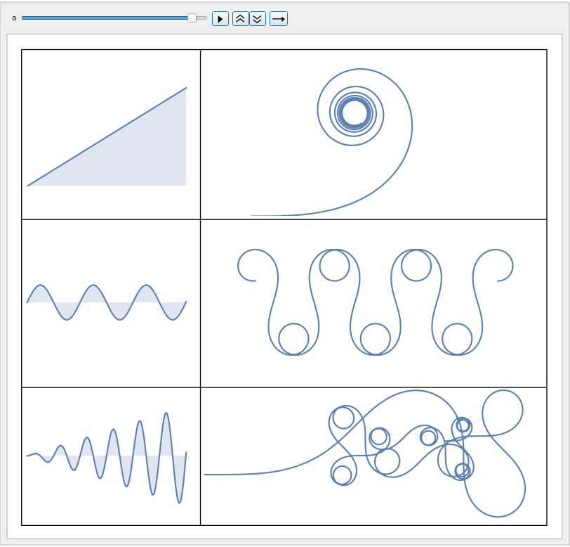
ssen5=IntFunc[sSin[2s],0];linear=IntFunc[s];linear2=IntFunc[5Cos[s]];Animate[Grid[{{Plot[s,{s,0,a},AxesFalse,PlotRange{{0,20},{0,20}},FillingAxis],ParametricPlot[{linear[[1]][s],linear[[2]][s]},{s,0,a/2},AxesFalse,PlotRange{{-.4,2.5},{0,1.4}},ImageSizeMedium]},{Plot[5Sin[s],{s,0,a},AxesFalse,PlotRange{{0,20},{-15,15}},FillingAxis],ParametricPlot[{linear2[[1]][s],linear2[[2]][s]},{s,0,a},AxesFalse,PlotRange{{-4,.6},{-1.4,.8}},ImageSizeMedium]},{Plot[sSin[2s],{s,0,a},AxesFalse,PlotRange{{0,20},{-20,20}},FillingAxis],ParametricPlot[{ssen5[[1]][s],ssen5[[2]][s]},{s,0,a},AxesFalse,PlotRange{{0,3.2},{-0.45,0.8}},ImageSizeMedium,MaxRecursion4]}},FrameAll],{a,0.001,20,0.001},AlignmentCenter,DefaultDuration40.]
Out[]=
Generating the curve
Generating the curve
IntFunc will return an InterpolatingFunction the coordinates x, y and ∫ f ds
In[]:=
intfuncs=IntFunc[s]
Out[]=
InterpolatingFunction
,InterpolatingFunction
,InterpolatingFunction


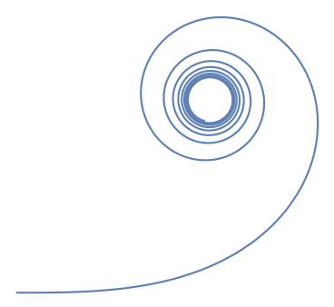
We can plot the curve directly with a parametric plot adding the dependence on [s]:
In[]:=
ParametricPlot[{intfuncs[[1]][s],intfuncs[[2]][s]},{s,0,10},AxesFalse,ImageSizeSmall]
Out[]=
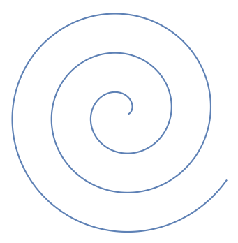
Other example is:
In[]:=
oversquareroot=IntFunc[1/Sqrt[s],.01];ParametricPlot[{oversquareroot[[1]][s],oversquareroot[[2]][s]},{s,0.1,100},AxesFalse,ImageSizeSmall]
Out[]=
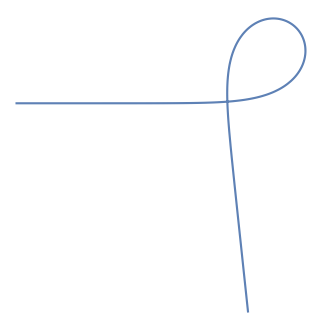
We can also plot the curve for a Gaussian Function, specifying the start and the end for the interpolation function:
In[]:=
gauss=IntFunc[Exp[-s^2+1],-4(*start*),4(*end*)];ParametricPlot[{gauss[[1]][s],gauss[[2]][s]},{s,-4,4},AxesFalse,ImageSizeSmall]
Out[]=
With the explicit coordinates of points we can plot them for a list of functions with the functions curve and curveplot, curve just find the explicit coordinates for the points with IntFunc and add the dependence of [s] to the interpolations functions that give us the coordinates of the points, on the other hand curveplot plots the curve in a parametric way.
curve[flist_,sta_,fin_]:=Module[{sol,soleval},sol=MapThread[IntFunc][{flist,ConstantArray[sta,Length[flist]],ConstantArray[fin,Length[flist]]}];soleval=Table[sol〚i,j〛[s],{i,Length[flist]},{j,2}]]curveplot[flist_,sta_,fin_]:=Module[{},MapThread[ParametricPlot][{flist,ConstantArray[{s,sta,fin},Length[flist]],ConstantArray[AxesFalse,Length[flist]],ConstantArray[ImageSizeTiny,Length[flist]]}]]
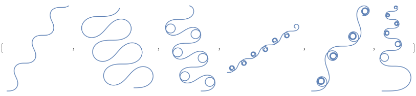
For example:
In[]:=
list={Sin[s],2Sin[s],5Sin[s],10Sin[s],10Sin[.6s],sSin[s]};sollist=curve[list,0.01,20];curveplot[sollist,0.01,20]
Out[]=
Database
Database
With the functions that allow us to automate the generatio of the curves for a lot of functions we generate a big database using a lot of different functions, you can see some of the curves here:
FeatureSpacePlot
FeatureSpacePlot
The FeatureSpacePlot function plots features extracted from the data as a scatter plot. We use it with some of the curves that we generate. We can see in it some regions, for example, the spirals are at the bottom, the complex curves are in the periphery and so on...
In a more general way the kind of curves that we can observe are:
In a more general way the kind of curves that we can observe are:
Functions that generate most of the curves
Functions that generate most of the curves
After the extense exploration we realize that you can get almost all kinds of curves with just 6 simple functions:
◼
a Sin[ b s ] + c when c=a and 0
◼
a s Sin[b s]
The only curves that you cannot get from these functions are the deformed spirals.
a Sin[ b s ] + c when c=a
a Sin[ b s ] + c when c=a
In this case the curves are bounded, i.e no matter how long we let the curve evolve, it will remain within a bounded subset.
a Sin[ b s ] + c when c=0
a Sin[ b s ] + c when c=0
These curves are un-bounded, when we let the curve evolve a long time , they won’t remain within a bounded subset, instead they will grow periodically.
-a/s^b with 1<b<0
-a/s^b with 1<b<0
In this case the curves are bounded, i.e when we compute them for longer times , they remain within a bounded subset, getting more and more dense as time increases.
a Exp[-s^2+b]
a Exp[-s^2+b]
These curves are un-bounded, when we let the curves evolve a long time, they won’t remain within a bounded subset. This is because the straight line will keep growing as time keeps advancing.
a Exp[-s^2] Sin [b s]
a Exp[-s^2] Sin [b s]
These curves are un-bounded, i.e when we let the curves evolve a long time, they won’t remain within a bounded subset, because the straight line keeps growing.
a s Sin[b s]
a s Sin[b s]
These curves are un-bounded, i.e when we let the curves evolve a long time, they won’t remain within a bounded subset, they will keep growing in radio and densitiy as the time advances.
a Sin[b s ] + a /s
a Sin[b s ] + a /s
These curves are un-bounded, i.e when we let the curves evolve a long time, they wont remain within a bounded subset. We will see with more detail what happens to them when we compute them for a longer time.
When we compute them for longer times the curves reveal their true stable form, i.e. spirals, with self-similar behaviour:
Conclusions
Conclusions
In this project we classify the shapes and curves defined by curvature obtained with different Arc Length functions. To do this we create the functions necessary to automate the creation of curves with local curvature based on different Arc Length functions. With these functions we did a parametric sweep through a wide range of values for different functions such as Trigonometrics, Exponentials, Polinomials, and others, in order to generate a database big enought to identify the feactures that can be used for classification among curves. After that we were able to identify the different kinds of curves that we can obtain from different functions, we run them for different times to see which ones where bounded or unbounded.
This reveals a really interesting behaviours of the curves, the most interestings ones where the “a Sin[b s ] + a /s” curves, since we can observe complex shapes, similar to the ones that we can observe in the nature.
And as we said before there is a lot yet to be explored, more functions, more parameters, and the possibility of having curves in 3D, which surely will offer very interesting results