CITE THIS NOTEBOOK: Bell's inequality, or why Nature is non-locally causal by Mads Bahrami. Wolfram Community MAR 11 2023.
[We] hope that even those who are not committed to such discussions will be convinced that Einstein has pointed out one of the most extraordinary property of Quantum Mechanics . We must thank J . Bell to have provided us with the possibility of experimentally evidencing this property.
In fact, since all of quantum computation is just and plainly an application of the quantum formalism, I do not see any reason whatsoever which might make it (a) superior to the quantum formalism itself or (b) of any use in overcoming the difficulties that physicists have met with it, in particular those which are at the basis of John Bell’s unsatisfaction with the theory.
What is the significance of these two quotes? One is from Allen Aspect, an experimental physicist who won the Nobel Prize in 2022, while the other is from a prominent theoretical physicist specializing in the foundations of quantum theory. Both of them were close friends of John. S. Bell. Together, these quotes capture the irony of the story I want to convey. My objective is to investigate Bell’s inequalities using the Wolfram quantum framework, utilizing the standard language of quantum computation (such as quantum gates, circuits, etc.) that is fully supported by this framework. Therefore, I highly suggest that my readers delve deeper into Bell’s seminal work (such as Bell’s theorem or inequalities) to understand the core idea and motivation behind his work, to the least. Here, I present a straightforward computational approach to comprehend the underlying mechanism of those equations, fully derived from quantum formalism, but with a new twist: quantum computation.
Entangled states, correlations, and measurement
Entangled states, correlations, and measurement
Let us consider a 2-qubit quantum system that is prepared in the following quantum state
In[]:=
ψm=QuantumState["PsiMinus"];ψm["Formula"]
Out[]=
|01〉
2
|10〉
2
As one can see, it is an entangled state
In[]:=
QuantumEntangledQ[ψm]
Out[]=
True
which is, of course, maximally entangled:
In[]:=
QuantumEntanglementMonotone[ψm]
Out[]=
1
An entangled state is a state that cannot be written as product of two states ⊗. This possibility can be tested using QuantumEntangledQ which returns as True or False.
ρ
1
ρ
2
Let’s define a unit vector in 3D (which is parametrized by two angles):
In[]:=
a[θ_,ϕ_]:={Sin[θ]Cos[ϕ],Sin[θ]Sin[ϕ],Cos[θ]}
Given two unit vectors, let’s find the angle between:
In[]:=
vecAngle=FullSimplify[VectorAngle[a[θ1,ϕ1],a[θ2,ϕ2]],Assumptions->{θ1∈Reals,θ2∈Reals,ϕ1∈Reals,ϕ2∈Reals}]
Out[]=
ArcCos[Cos[θ1]Cos[θ2]+Cos[ϕ1-ϕ2]Sin[θ1]Sin[θ2]]
Now let us calculate the quantum expectation/mean value of a composite operator as follows: with with the Pauli vector.
〈|.⊗.|〉
-
ψ
a
1
σ
a
2
σ
-
ψ
|〉=(|01〉-|10〉)
-
ψ
1
2
σ
Define a Pauli vector:
In[]:=
σ[θ_,ϕ_]:=QuantumOperator[a[θ,ϕ].Table[PauliMatrix[i],{i,3}]]
Calculate :
〈|.⊗.|〉
-
ψ
a
1
σ
a
2
σ
-
ψ
In[]:=
ψm["Dagger"][QuantumTensorProduct[σ[θ1,ϕ1],σ[θ2,ϕ2]][ψm]]
Out[]=
QuantumState


Note that the result is a scalar, but as an object, we treat it as a quantum state object, with 0 number of qudits (look at the summary box of above result). The actual scalar number can be extracted like this:
In[]:=
Φ12=FullSimplify[Normal[%[[1,1]]]]
Out[]=
-Cos[θ1]Cos[θ2]-Cos[ϕ1-ϕ2]Sin[θ1]Sin[θ2]
One can show that the expectation value is related to the vector angle as follows:
In[]:=
-Cos[vecAngle]==Φ12
Out[]=
True
In other words:
Remember this result. We will use it later within Bell’s inequality. But before jumping to Bell’s inequality, let’s explore how above expectation value can be calculated or obtained experimentally using quantum circuits.
〈|.⊗.|〉=-cos()
-
ψ
a
1
σ
a
2
σ
-
ψ
Φ
12
Remember this result. We will use it later within Bell’s inequality. But before jumping to Bell’s inequality, let’s explore how above expectation value can be calculated or obtained experimentally using quantum circuits.
For simplicity, let’s consider the case where qubit-1 is measured in Pauli-X basis, and qubit-2 in another basis which obtained by rotating Pauli-X basis by π/8 around z-axis
Define new basis (Pauli-X which is rotated by π/8 around z-axis):
In[]:=
newBasis=N@QuantumOperator[{"RZ",π/8}][QuantumBasis["X"]];
Note I added N, just to enforce numeric calculations, which are faster.
Measure in Pauli-X basis on qubit-1, in new basis on qubit-2, when the system is prepared in :
-
ψ
In[]:=
meas=QuantumMeasurementOperator["X"]@QuantumMeasurementOperator[newBasis,{2}]@QuantumState["PsiMinus"];
Find the measurement probabilities:
In[]:=
prob=meas["Probabilities"]
Out[]=
00.0190301,10.48097,00.48097,10.0190301
ψ
x
-
ψ
x
-
ψ
x
+
ψ
x
+
Note the first and last results correspond to + eigenvalue (their multiplication) and middle ones -. So for the mean value, we do as follows:
In[]:=
prob[[1]]+prob[[4]]-(prob[[2]]+prob[[3]])
Out[]=
-0.92388
Taking of above result (note ) one can confirm:
-1
cos
〈|.⊗.|〉=-cos()
-
ψ
a
1
σ
a
2
σ
-
ψ
Φ
12
In[]:=
ArcCos[-%]==π/8
Out[]=
True
which is what we expected. Now let’s focus on the circuit version.
The following quantum circuit prepare a 2-qubit quantum system in first, and then two measurements are performed on 2-qubits (as described previously).
-
ψ
In[]:=
qc1=QuantumCircuitOperator[{QuantumCircuitOperator[{"X"->{1,2},"H","CNOT"},"Circuit to create "],{"RZ",π/8}->2,"H"->{1,2},{1},{2}}];qc1["Diagram"]
-
ψ
Out[]=
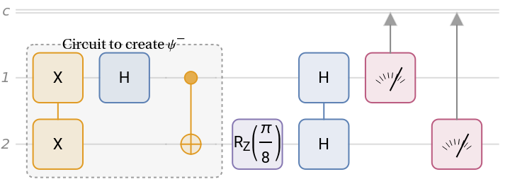
The above circuit is the one you see in many literatures, mostly because that is how you send it to a Quantum Processing Unit (QPU, ie a quantum hardware). However, in our framework, you can define the measurement in any basis, for example:
In[]:=
qc2=QuantumCircuitOperator[{QuantumCircuitOperator[{"X"->{1,2},"H","CNOT"},"Circuit to create "],QuantumMeasurementOperator["X"],QuantumMeasurementOperator[newBasis,{2}]}];qc2["Diagram"]
-
ψ
Out[]=
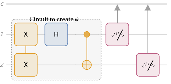
Note that those light purple boxes representing measurement are fundamentally different from other boxes representing usual gates. But that is a different story (refer to this for more details).
Circuits qc1 and qc2 are equivalent. However, for the sake of communicating with a QPU, some transpilers may have some issues with defining measurements for qc2. So let’s focus on first circuit:
In[]:=
qc1["Diagram"]
Out[]=
In above circuit, ->{θ=π/2,ϕ=0} (measurement on qubit-1) and ->{θ=π/2,ϕ=π/8} (measurement on qubit-2). Note the Hadamard (H) boxes before measurements are transforming the measurement to Pauli-X, and rotation rotates it by an angle in xy-plane. So the correlation function should be
a
1
a
2
R
z
-cos(π/8)
Find the probabilities from above circuit:
In[]:=
prob1=FullSimplify/@qc1[]["Probabilities"]
Out[]=
00,011+Cos,101+Cos,11
1
2
2
Sin
π
16
1
4
π
8
1
4
π
8
1
2
2
Sin
π
16
Calculate the correlation function:
In[]:=
prob1[|00〉]+prob1[|11〉]-(prob1[|01〉]+prob1[|10〉])//FullSimplify
Out[]=
-Cos
π
8
which is, of course, what we expected.
Note that the experimental results that one gets out of a QPU is counters per measurement results; something like this:
In[]:=
exp=qc1[]
Out[]=
QuantumMeasurement

Simulate measurement results for 1024 shots:
In[]:=
counts=Counts[exp["SimulatedMeasurement",1024]]
Out[]=
|10〉492,|01〉504,|11〉15,|00〉13
Calculate the corresponding correlation (using frequency of occurrence for each result):
In[]:=
counts[|00〉]+counts[|11〉]-(counts[|01〉]+counts[|10〉])
1024
which is what we expected (close enough, given number of shots)
Now let’s see how those correlations are used in Bell inequality
Bell’s inequality
Bell’s inequality
There are many good literature on the Bell’s inequality and what it implies. I guess by looking at the title of this notebook, you have an idea how I understand that. If you are looking for a short paper, with some nice [personal] history, I highly recommend this preprint by GianCarlo Ghirardi: John Stuart Bell: recollections of a great scientist and a great man.
I had the pleasure of many interactions and discussions with GianCarlo, when I was in Trieste, Italy, doing my grad studies. GianCarlo sadly passed away prematurely, like the great John Bell, himself.
Let me rephrase the reasoning behind the derivation of Bell’s inequality (following Ghirardi):
“Experimental Perfect Correlations” ∧ “Bell’s Locality” “Determinism”
“Determinism” ∧ “Bell’s Locality” “Bell’s Inequality”
“General Quantum Correlations” ¬ “Bell’s Inequality”
¬“Bell’s Inequality” ¬ “Determinism” ∨ ¬“Bell’s Locality”
Summarizing: “Natural Processes” ¬“Bell’s Locality”, i.e.: Nature is non-locally causal.
“Determinism” ∧ “Bell’s Locality” “Bell’s Inequality”
“General Quantum Correlations” ¬ “Bell’s Inequality”
¬“Bell’s Inequality” ¬ “Determinism” ∨ ¬“Bell’s Locality”
Summarizing: “Natural Processes” ¬“Bell’s Locality”, i.e.: Nature is non-locally causal.
Well, if anything, let me comment on Bell’s Locality, which implies that measurement probabilities (accessible or not, to observer) at two space-like regions are independent.
One can obtain those regions (where the Bell’s inequality is violated) explicitly:
One can also find the maximum violation, which happens at π/4:
Explore Bell’s inequality in a quantum circuit
Explore Bell’s inequality in a quantum circuit
Now let’s calculate the corresponding correlations, using above circuits. I will find those correlations analytically, using our quantum framework.
Of course, one can find the numerical value of those correlations (theoretically, by some simulation as shown in the previous section, or experimentally using some QPUs).
Of course, one can find the numerical value of those correlations (theoretically, by some simulation as shown in the previous section, or experimentally using some QPUs).
Plug them into Bell’s inequality:
Plot the region that Bell’s inequality (above) is violated:
Certainly, the aforementioned circuits may be executed using existing QPUs to obtain empirical correlations. However, in my personal opinion, such findings hold little value unless we know the details of experimental setting employed, to address problems commonly known as “loopholes” (such as the locality loophole). To the best of my knowledge, these details are largely disregarded by the quantum computation community, mostly because details of experimental design (e.g., topology of qubits) are only relevant as far as circuit design (e.g., what controlled gates one can have); which is understandable. However, this is reminiscent of the quote by GianCarlo Ghirardi regarding quantum computations and quantum foundations at the beginning of this essay. I believe that this issue is a reflection of the human element in research, and I cannot identify any scientific justification for this trend. However, this is a separate issue that is beyond the scope of this essay.
Initialization cells
Initialization cells
Install the quantum paclet first