Consider the closed loop shown in Figure 11.8 in [1]where =, =, =, =1, and =1+. Here, we consider a proportional-integral controller since we have =1+. We propose to set the value of the control gain for a fixed integral time (=5).
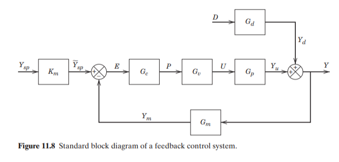
G
p
1
5s+1
G
v
1
2s+1
G
m
1
s+1
K
m
G
c
K
c
1
5s
G
c
K
c
1
5s
K
c
τ
I
The closed-loop transfer function for step point changes is given by (if =0). When a disturbance is applied (i.e. ), the response is plotted and values of the three integral errors are given below.
G==
Y
D
5s(1+s)(1+2s)
(1+10s)(Kc+5s(1+s)(1+2s))
Y
sp
D=
1
s
y(t)
These three integral errors (all truncated at in the calculation shown here) are defined by: (the integral of the absolute value of the error indicated by the gray area shown in the response versus time plot), (the integral of the squared error),and (the integral of the time-weighted absolute error).
t=2000
IAE=e(t)dt
∞
∫
0
ISE=dt
∞
∫
0
2
(e(t))
ITAE=te(t)dt
∞
∫
0
Controller tuning is performed by computing the values of that minimize the integral errors. These values are indicated by blue dots.
K
c
Closed-looptransferfunctionis

5s(1+s)(1+2s)
(1+10s)(Kc+5s(1+s)(1+2s))
In[]:=
Kc=.
In[]:=
Gp=1/(5s+1);Gv=1/(2s+1);Gm=1/(s+1);Gd=1/(10s+1);Gc=Kc(1+1/(5s));
In[]:=
Gd/(1+GcGvGpGm)//FullSimplify
Out[]=
5s(1+s)(1+2s)
(1+10s)(Kc+5s(1+s)(1+2s))
Time-domain response
In[]:=
y[q_?NumericQ]:=InverseLaplaceTransform1s,s,t//Chop;(*q=Kc*)
5s(1+s)(1+2s)
(1+10s)(q+5s(1+s)(1+2s))
In[]:=
ym[q_?NumericQ]:=InverseLaplaceTransform1sGm,s,t//Chop;(*q=Kc*)
5s(1+s)(1+2s)
(1+10s)(q+5s(1+s)(1+2s))
Below we compute the three integral errors
Below we compute the three integral errors
In[]:=
f1[q_?NumericQ]:=Re[Quiet@NIntegrate[Abs[ym[q]],{t,0,2000},AccuracyGoal->10]//Chop];(*IAE*)f2[q_?NumericQ]:=Re[Quiet@NIntegrate[(ym[q])^2,{t,0,2000},AccuracyGoal->10]//Chop];(*ISE*)f3[q_?NumericQ]:=Re[Quiet@NIntegrate[tAbs[ym[q]],{t,0,2000},AccuracyGoal->10]//Chop];(*ITAE*)
In[]:=
Kc=.
In[]:=
IAEdata=Join[Flatten[{{{Kc,IAE}},Table[{q,f1[q]},{q,1,6.5,0.1}]},1]]
Out[]=
{{Kc,IAE},{1.,5.},{1.1,4.54545},{1.2,4.16667},{1.3,3.84615},{1.4,3.57143},{1.5,3.33333},{1.6,3.125},{1.7,2.94118},{1.8,2.77778},{1.9,2.63158},{2.,2.5},{2.1,2.38095},{2.2,2.27273},{2.3,2.17391},{2.4,2.08333},{2.5,2.00415},{2.6,1.93755},{2.7,1.87768},{2.8,1.82946},{2.9,1.7874},{3.,1.7453},{3.1,1.72945},{3.2,1.7054},{3.3,1.68813},{3.4,1.66385},{3.5,1.66351},{3.6,1.63887},{3.7,1.65091},{3.8,1.65871},{3.9,1.66307},{4.,1.67034},{4.1,1.68097},{4.2,1.69469},{4.3,1.70758},{4.4,1.73169},{4.5,1.75692},{4.6,1.7329},{4.7,1.8166},{4.8,1.87645},{4.9,1.93529},{5.,1.93436},{5.1,2.05326},{5.2,2.03216},{5.3,2.09519},{5.4,2.16308},{5.5,2.2384},{5.6,2.33465},{5.7,2.42804},{5.8,2.53528},{5.9,2.66065},{6.,2.80242},{6.1,2.96953},{6.2,3.16226},{6.3,3.38785},{6.4,3.65645},{6.5,4.00587}}
In[]:=
%//TableForm
Out[]//TableForm=
Kc | IAE |
1. | 5. |
1.1 | 4.54545 |
1.2 | 4.16667 |
1.3 | 3.84615 |
1.4 | 3.57143 |
1.5 | 3.33333 |
1.6 | 3.125 |
1.7 | 2.94118 |
1.8 | 2.77778 |
1.9 | 2.63158 |
2. | 2.5 |
2.1 | 2.38095 |
2.2 | 2.27273 |
2.3 | 2.17391 |
2.4 | 2.08333 |
2.5 | 2.00415 |
2.6 | 1.93755 |
2.7 | 1.87768 |
2.8 | 1.82946 |
2.9 | 1.7874 |
3. | 1.7453 |
3.1 | 1.72945 |
3.2 | 1.7054 |
3.3 | 1.68813 |
3.4 | 1.66385 |
3.5 | 1.66351 |
3.6 | 1.63887 |
3.7 | 1.65091 |
3.8 | 1.65871 |
3.9 | 1.66307 |
4. | 1.67034 |
4.1 | 1.68097 |
4.2 | 1.69469 |
4.3 | 1.70758 |
4.4 | 1.73169 |
4.5 | 1.75692 |
4.6 | 1.7329 |
4.7 | 1.8166 |
4.8 | 1.87645 |
4.9 | 1.93529 |
5. | 1.93436 |
5.1 | 2.05326 |
5.2 | 2.03216 |
5.3 | 2.09519 |
5.4 | 2.16308 |
5.5 | 2.2384 |
5.6 | 2.33465 |
5.7 | 2.42804 |
5.8 | 2.53528 |
5.9 | 2.66065 |
6. | 2.80242 |
6.1 | 2.96953 |
6.2 | 3.16226 |
6.3 | 3.38785 |
6.4 | 3.65645 |
6.5 | 4.00587 |
In[]:=
ISEdata=Join[Flatten[{{{Kc,ISE}},Table[{q,f2[q]},{q,1,6.2,0.1}]},1]]
Out[]=
{{Kc,ISE},{1.,1.10519},{1.1,0.958807},{1.2,0.841654},{1.3,0.746316},{1.4,0.667618},{1.5,0.601852},{1.6,0.546301},{1.7,0.498934},{1.8,0.458209},{1.9,0.422932},{2.,0.392174},{2.1,0.365194},{2.2,0.341404},{2.3,0.320325},{2.4,0.301567},{2.5,0.28481},{2.6,0.269789},{2.7,0.256283},{2.8,0.244105},{2.9,0.2331},{3.,0.223133},{3.1,0.214092},{3.2,0.205879},{3.3,0.198413},{3.4,0.19162},{3.5,0.18544},{3.6,0.179818},{3.7,0.17471},{3.8,0.170075},{3.9,0.165879},{4.,0.162094},{4.1,0.158693},{4.2,0.155657},{4.3,0.152968},{4.4,0.150612},{4.5,0.148579},{4.6,0.146861},{4.7,0.145454},{4.8,0.144358},{4.9,0.143574},{5.,0.14311},{5.1,0.142974},{5.2,0.143182},{5.3,0.143754},{5.4,0.144717},{5.5,0.146104},{5.6,0.147959},{5.7,0.150337},{5.8,0.153307},{5.9,0.156961},{6.,0.161411},{6.1,0.16681},{6.2,0.173354}}
In[]:=
%//TableForm
Out[]//TableForm=
Kc | ISE |
1. | 1.10519 |
1.1 | 0.958807 |
1.2 | 0.841654 |
1.3 | 0.746316 |
1.4 | 0.667618 |
1.5 | 0.601852 |
1.6 | 0.546301 |
1.7 | 0.498934 |
1.8 | 0.458209 |
1.9 | 0.422932 |
2. | 0.392174 |
2.1 | 0.365194 |
2.2 | 0.341404 |
2.3 | 0.320325 |
2.4 | 0.301567 |
2.5 | 0.28481 |
2.6 | 0.269789 |
2.7 | 0.256283 |
2.8 | 0.244105 |
2.9 | 0.2331 |
3. | 0.223133 |
3.1 | 0.214092 |
3.2 | 0.205879 |
3.3 | 0.198413 |
3.4 | 0.19162 |
3.5 | 0.18544 |
3.6 | 0.179818 |
3.7 | 0.17471 |
3.8 | 0.170075 |
3.9 | 0.165879 |
4. | 0.162094 |
4.1 | 0.158693 |
4.2 | 0.155657 |
4.3 | 0.152968 |
4.4 | 0.150612 |
4.5 | 0.148579 |
4.6 | 0.146861 |
4.7 | 0.145454 |
4.8 | 0.144358 |
4.9 | 0.143574 |
5. | 0.14311 |
5.1 | 0.142974 |
5.2 | 0.143182 |
5.3 | 0.143754 |
5.4 | 0.144717 |
5.5 | 0.146104 |
5.6 | 0.147959 |
5.7 | 0.150337 |
5.8 | 0.153307 |
5.9 | 0.156961 |
6. | 0.161411 |
6.1 | 0.16681 |
6.2 | 0.173354 |
The minimal values of IAE, ISE and ITAE and their corresponding values of q = Kc
Below we plot the three integral errors and we indicate with a blue dot the optimal values of Kc (the PI controller’s gain)
Below we plot the three integral errors and we indicate with a blue dot the optimal values of Kc (the PI controller’s gain)
Below we plot the response for Kc=3.25, 2.75 and 7.5
References
References
[1] D. E. Seborg, T. F. Edgar, D. A. Mellichamp, and F. J. Doyle III, Process Dynamics and Control, 4th ed., Hoboken, NJ: John Wiley & Sons, Inc., 2017.
CITE THIS NOTEBOOK
CITE THIS NOTEBOOK
Controller design for disturbance rejection
by Housam Binous and Ahmed Bellagi
Wolfram Community, STAFF PICKS, March 22, 2024
https://community.wolfram.com/groups/-/m/t/3146113
by Housam Binous and Ahmed Bellagi
Wolfram Community, STAFF PICKS, March 22, 2024
https://community.wolfram.com/groups/-/m/t/3146113