Wolfram Cloud Document

There are many algorithms for diagnosing chaos. The most famous are Lyapunov exponent and correlation dimension. But they require a lot of computation and knowledge of many details. By chance I found a rather old article that suggests effective and a well thought-out chaos analysis method, which returns the result in 0-1 format. Although the idea of describing chaos by one number is a bit speculative, it can be useful for a rough evaluation of various processes' behavior . This algorithm is perfectly implemented in the Wolfram Language as short fast code (and I’m sure it can still be optimized).

Short theory

Authors consider the sequences of sums

(n)=

∑

j=1

sin(jc)

and

(n) =

∑

j=1

cos(jc)

, where

, 1 ≤ j ≤ N are observations data and 0 < c < π - some parameter. In fact this is kind of AnglePath. Then calculate mean square displacement

(n)=1/N

∑

j=1

(

(j+n)-

(j))

(

(j+n)-

(j))

for a large number n, but still n ≪ N. By the slope of the

plot one can already get an idea of the degree of data chaos.But the authors recommend performing additional calculations, obtaining a normalized value of 0 <

< 1, where 0 is for absolutely regular (e.g., periodic) and 1 is for completely random data. In general, the method is a synthesis of spectral analysis and evaluation of random walks.Parameter c can be considered a resonance frequency. Pseudo-random observations can show resonances at certain frequencies giving small

, so the final result is a median of

values of

for different c.

Main code

Literal implementation of the article's algorithm, using cool built-ins. κ stands for c in paper, ν =

max

and chaosValue is

itself.

Clear[chaosValue,safeCorr];(*Thedatamayaccidentallybeaconstantarray,andthiscancauseanerrorinCorrelation*)safeCorr[x_,y_]:=With[{cov=Covariance[x,y],sd=StandardDeviation/@{x,y}},If[AnyTrue[sd,PossibleZeroQ],-1,cov/sd[[1]]/sd[[2]]]];chaosValue[data_,κ_,ν_:0.1]:=ModulelenData=Length@data,rngN=Range@(1+⌈νLength@data⌉),μ=

(Mean@data)

(1-Cos@κ),pq,pq=Rest@Block[{i=0},FoldList[(i++;{#1[[1]]+#2Sin[κi],#1[[2]]+#2Cos[κi]})&,{0,0},data]];safeCorr[rngN,Total[Flatten[pq[[;;lenData-#]]-pq[[#+1;;lenData]]]^2]/lenData-μ(1-Cos[#κ])&/@rngN];

Simple 0 - 1 test

The authors propose to select ~100 samples for κ in the range π/5 < κ < 4π/5 and take median of all

. We will need more detailed data, so the following code provides settings:

In[]:=

Clear[chaosTestList];chaosTestList[data_,ν_:0.1,mn_:π/5,mx_:4π/5.,nums_:100]:=ParallelTable[chaosValue[data,κ,ν],{κ,Subdivide[mn,mx,nums]}];

Classic example

Let’s check the implementation on the well known example: logistic map.

Clear[logGen];logGen[p_,num_:2000]:=NestList[p#(1-#)&,RandomReal[],num];

Very desirable to perform parallel computations (in accordance with your hardware)

In[]:=

LaunchKernels[];

Build a plot of medians chaosTestList for different logistic map parameters. For the specified parameters evaluation may take 15-20 sec. User can get more detailed picture, changing them.

In[]:=

logMedians=Block[{semps=Subdivide[3.5,4.,100],i=1},PrintTemporary[ProgressIndicator[Dynamic@i,{1,100}]];Table[i++;Median@chaosTestList@logGen@s,{s,semps}]];

Framed@ListLinePlot[logMedians,PlotLabel"Chaos test value for logistic map",AxesLabel{"Map\n param","Median"},PlotStyle->Thickness@0.005,Mesh->All,MeshStyle->Directive[PointSize@0.01,Brown],PlotRange->{-0.5,1},DataRange{3.5,4.},ImageSize->300]

Out[]=

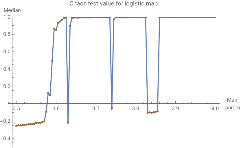
We see well known pattern of transition to randomness, with windows of stability within the area of chaos.

Generalization

The medians disadvantage is low sensitivity at 0.9 < K < 1. Let's use Lehmer mod generator, which allows to get any degree of chaos.

In[]:=

Clear[modGen];modGen[p_,num_:4000]:=Standardize[N@NestList[Mod[Prime[p]#,Prime[p+13]]&,Prime[p+7],num]];

Compare the results of iterations for different prime modulo (and for built-in RandomReal). We use more samples of κ , 0 < κ < π and add value of interquartile range IQR.

modSeeds={84,212,420};modData=chaosTestList[#,0.1,1./600,π,600]&/@Append[modGen/@modSeeds,RandomReal[{-1,1},4000]];

In[]:=

modLbls=MapThread[Style[StringForm["p: ``, median: ``, IQR: ``",#1,Round[#2,.001],Round[#3,.002]],10,Brown,Bold]&,{Append[modSeeds,"rnd"],Median/@modData,InterquartileRange/@modData}];

In[]:=

Grid[Partition[MapThread[ListLinePlot[#1,PlotLabel#2,AxesLabel{"κ","K"},PlotStyle->Thickness@0.005,Mesh->All,MeshStyle->Directive[PointSize@0.01,Brown],PlotRange->{0.,1.},DataRange{0.,π},ImageSize->200]&,{modData,modLbls}],2],Frame->All]

Out[]=

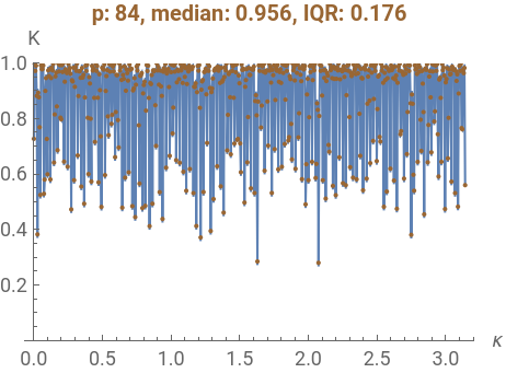
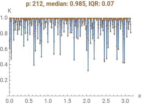
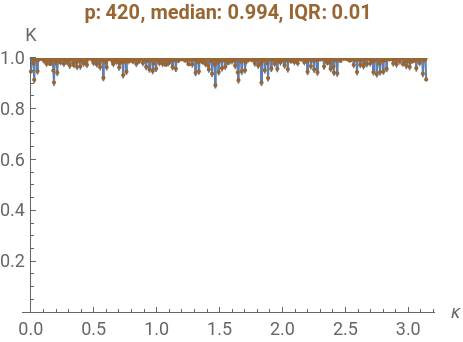
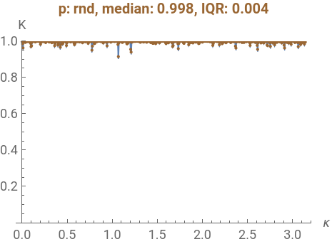
We see that the behaviour of generators is markedly different, resonances have various degrees of density and depth. Meanwhile, the final median values differ very little; but IQR values are much more indicative.

Substitution systems: the edge of chaos

My favorite mathematical objects are substitution systems. I have described how to generate, select and display them here. Using the utilities from these notebooks and the test presented here, we will do a small study.

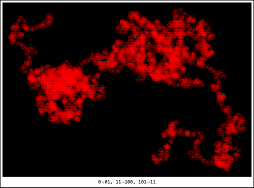
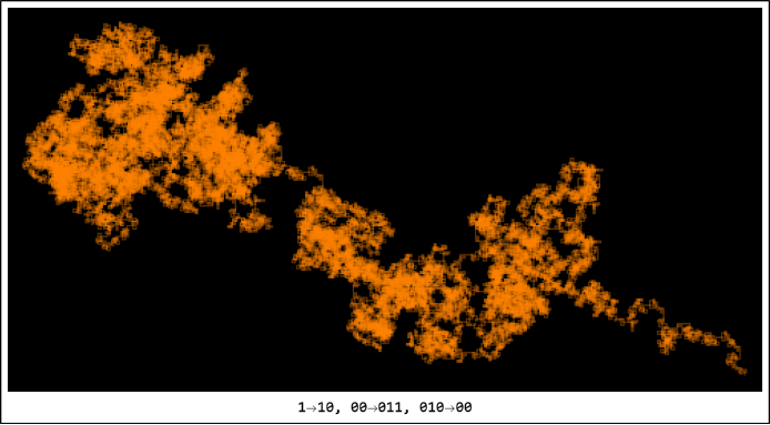
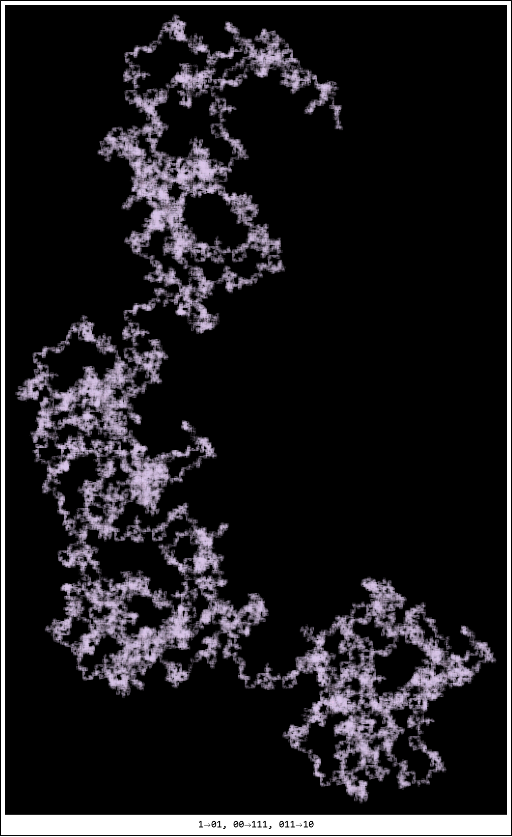
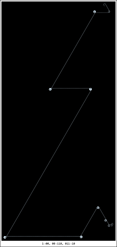
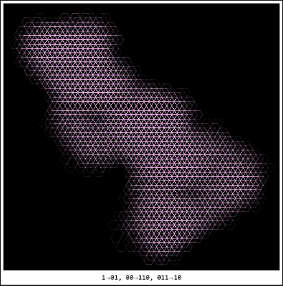
Consider the rule signature {{1, 2}, {2, 3}, {3, 2}}. Select the correct and non-periodic. They will be 2280. With chaos test we calculate medians and IQR of long enough generated sequences. At the beginning we will look at the candidates for the most chaotic:

Rule	Median	IQR
001, 11100, 10111	0.997	0.0065
110, 00011, 01000	0.997	0.0065
010, 11000, 10001	0.996	0.01

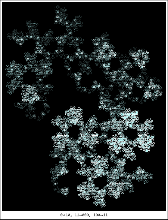
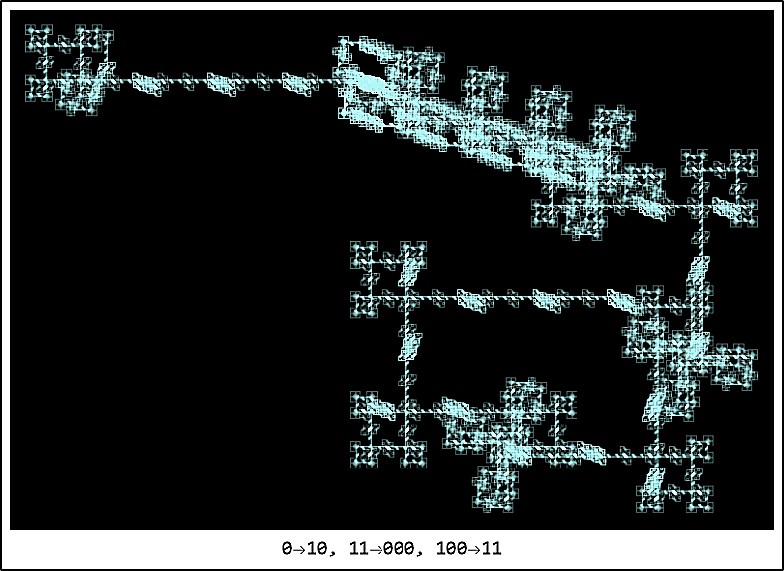
Turtle graphic for binary sequences generated by these rules are typical Rozy fractals:

But we can pick rules with a smaller median value and a larger one - IQR. So we can find artifacts lying on the edge of chaos and exhibiting unusual behavior.Rule 100, 00110, 01110, median 0.878, IQR 0.102:

(Levy flights)Rule 101, 00110, 01110, median 0.948, IQR 0.19:

And finally, the most interesting thing I found this time. Rule 010, 11000, 10011, median 0.985, IQR 0.063, turtle graphics for π/3 and π/2:

CITE THIS NOTEBOOK

Smart 0-1 chaos test: applications to modular generators, substitution rules, and Rozy fractals
by Denis Ivanov
Wolfram Community, STAFF PICKS, May 1, 2025
https://community.wolfram.com/groups/-/m/t/3453762