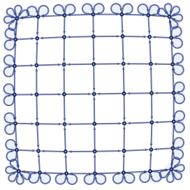
The following is an algorithm and a hypergraph rewriting ruleset that produces a single-connected square grid.
How is this different from existing grid-making rulesets? This one is designed, not “discovered”. The space unfolds in clear stages, and produces a regular grid; the rules are human-readable.
What value does this bring? While the algorithm itself is straightforward, programming it as a hypergraph rewriting ruleset is challenging. Rule misapplication is ubiquitous. Enforcement of an execution order is non-trivial. The only debugging tool is “trial and error”.
With this post, I want to spell out my solutions and thus provide guidance to those who might want to construct their own universes.
Why was this made? For fun. I’d like to make a bare-bones universe, consisting only of space and basic particle interactions – and this is the first step to it.
Ruleset
Ruleset
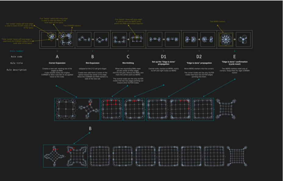
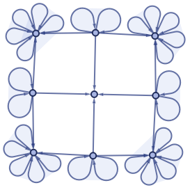
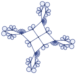
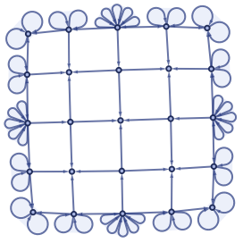
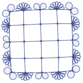
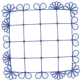
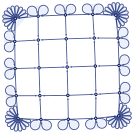
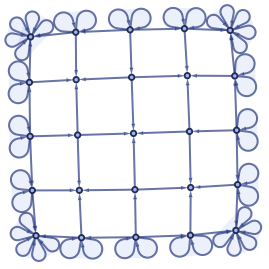
We have a rectangular space with four corners. Let’s differentiate it into two zones: “outer layer” (active) and “inside” (done). First, to each corner of the outer layer, add a new cell. Second, fill the gaps between the expanded corners. Third, reset the cycle resets.
The algorithm executes these three steps in order – that’s an unnecessary restriction, enforced for aesthetic reasons: without it, the growth of the corners will outpace the growth of the inner area, which leads to unappealing “tendrils”.
The algorithm executes these three steps in order – that’s an unnecessary restriction, enforced for aesthetic reasons: without it, the growth of the corners will outpace the growth of the inner area, which leads to unappealing “tendrils”.
Key ideas:
1
.Algorithm-specific information is stored with self-loops and edge patterns. For example, {x,x,x} marks an outer layer node – so if the rule needs to be applied only to the outer layer, it can reference this marker and avoid misapplication.
2
.Aliasing: OUTER[x,y] = {x,x,x}, {y,y,y} – this drastically improves readability and eases the editing. I personally had a lot of trouble with edge alignment in patterns – so being able to encapsulate that in CELL[...] and then use both in input and output of the rules removed a lot of typo-based bugs for me.
3
.Rule execution order is enforced by adding extra markers. For example, Rule A is dependent on having both OUTER and CORNER markers, and produces the RIMs – which are needed by Rules B and C. Rule A also moves apart the OUTERs and CORNERs – which blocks it from execution until other rules bring them back.
4
.Accounting for symmetry. Our square space is symmetrical at four axes, which breaks it into eight equivalent sectors. Creating rules that are contained within a single sector is crucial for preventing rule misapplication.
Code
Code
(*v2,attemptingtocleanstuff*)OUTER[arg_]:={arg,arg,arg}OUTER[args__]:=Splice[Map[OUTER,{args}]]CORNER[arg_]:={arg,arg,arg,arg}CORNER[args__]:=Splice[Map[CORNER,{args}]]RIM[arg_]:={arg,arg,arg,arg,arg}RIM[args__]:=Splice[Map[RIM,{args}]]MERG[arg_]:={arg,arg,arg,arg,arg,arg}MERG[args__]:=Splice[Map[MERG,{args}]]cell[in1_,out2_,in2_,out1_]:=Splice[{{out1,in1},{out1,in2},{out2,in1},{out2,in2}}]incell[mid1_,out_,mid2_,in_]:=Splice[{{mid1,in},{mid2,in},{out,mid1},{out,mid2}}]line[l1_,l2_,l3_]:=Splice[{{l1,l2},{l2,l3}}]nodup[args__]:=Splice[DeleteDuplicates[{args}]]rule={(*1.StepA:Expandcorners(thiscreatesrims)*){OUTER[x],CORNER[x]}{CORNER[x,x],cell[c,b,x,a],OUTER[c],RIM[a,b]},(*2.StepB:Expandrimsfromthecornertowardthecenteroftheedge(torimswilltouchthere).Note–thisdoesn'thappenfor3x3grid*){RIM[l4],CORNER[l3],OUTER[l2,l1],line[l1,l2,l3],{l4,l3}}{RIM[a],CORNER[l2],OUTER[l4,l1],line[l1,l2,l3],{a,l2},{a,l4},{l4,l3}},(*3.StepC:Knittouchingrims(andmarktheknitpointasMERG)*){RIM[l2,r2],CORNER[l1,r1],OUTER[x],{l2,l1},{x,l1},{x,r1},{r2,r1}}{OUTER[l2,r2],MERG[a],nodup[incell[l2,a,x,l1],incell[r2,a,x,r1]]},(*4.StepD1:StartmovingtheMERGmarkersbacktowardthecorners*){MERG[x],OUTER[y,z],{x,y},{x,z}}{MERG[y,z],OUTER[x,y,z],{x,y},{x,z}},(*5.StepD2:PropagateMERGmarkertowardthecorners*){MERG[x],OUTER[x,y],{x,y}}{MERG[y],OUTER[x,y],{x,y}},(*6.StepE:WhentwoMERGmarkersmeet,thatmeanstheyreachedacorner(thisresetscurrentexpansioncycle)*){MERG[x,x]}{CORNER[x]}};initState={{2,1},{3,1},{4,1},{5,1},{2,6},{2,7},{3,7},{3,8},{4,8},{4,9},{5,9},{5,6},OUTER[2,3,4,5,6,7,8,9],CORNER[6,7,8,9]};steps=16;evolution=[rule,initState,steps];RulePlot[evolution]evolution["StatesPlotsList"]evolution["AllEventsRuleIndices"]
Out[]=

Out[]=
,
,
,
,
,
,
,
,
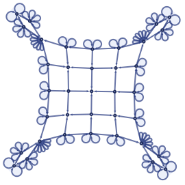
,
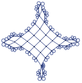
,
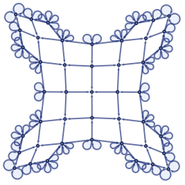
,
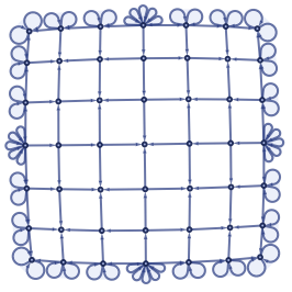
,
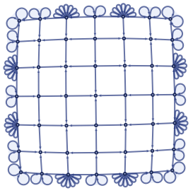
,
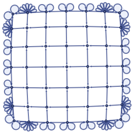
,
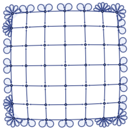
,
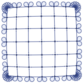
,
Out[]=
{1,1,1,1,3,3,3,3,4,4,4,4,5,5,5,5,5,5,5,5,6,6,6,6,1,1,1,1,2,2,2,2,2,2,2,2,3,3,3,3,4,4,4,4,5,5,5,5,5,5,5,5,5,5,5,5,5,5,5,5,6,6,6,6,1,1,1,1}
Other notes
Other notes
Extension vs subdivision. Expansion of this universe is achieved by extension – which means that any two nodes in the “stable” inside area remain forever near each other. Contrast that with an idea of subdivision, when the space expands by adding a new node between two existing ones: node-sized particles would be pulled apart and the bigger-sized matter would be shredded – unless some pulling force would be constantly updating it and pulling together. This makes me think about our universe expanding and the existence of gravitation and other fundamental interactions.
Algorithm side effects as proto-particles. Below I link a previous version of the algorithm, that leaves “junk” during its execution. I like to think of them as the matter created during the space unfolding (although, I was unable to create a rule that can operate over them without breaking the expansion).
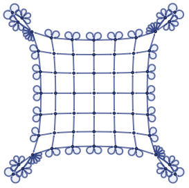
“Aberrant Fringes”. It is interesting, that the outer layer is almost separate reality from the other space: with its own unique structures and rules that apply nowhere else.
Proper 2D. In my code, the space is single-connected (two nodes share one directional edge). For a double connection, one would need extra markers to differentiate corners and edge-midpoints (now, they are marked with all in-pointing and all out-pointing vertices respectively). For that, one might use an extra edge on the outer layer, that would be removed during the expansion.
Negation is not available. Markers like {x,x,x} cannot be used to indicate the absence of something. If you do not include it in a rule, that rule will apply both to the patterns with it and without it. Absence needs to be either indicated with its own markers – or derived from the pattern outside.
Older ruleset, with side effects
Older ruleset, with side effects
OUTER[arg_]:={arg,arg,arg}OUTER[args__]:=Splice[Map[OUTER,{args}]]CORNER[arg_]:={arg,arg,arg,arg}CORNER[args__]:=Splice[Map[CORNER,{args}]]RIM[arg_]:={arg,arg,arg,arg,arg}RIM[args__]:=Splice[Map[RIM,{args}]]cell[in1_,out2_,in2_,out1_]:=Splice[{{out1,in1},{out1,in2},{out2,in1},{out2,in2}}]incell[mid1_,out_,mid2_,in_]:=Splice[{{mid1,in},{mid2,in},{out,mid1},{out,mid2}}]line[l1_,l2_,l3_]:=Splice[{{l1,l2},{l2,l3}}]nodup[args__]:=Splice[DeleteDuplicates[{args}]]{rect1,rect2}={incell,cell};rule={(*Inrules2and3there'sinverseconnectionbetweenproducedcellformatin2andinputcellformatin3:if2usesincell,3mustusecell–coverbyusingofrect1andrect2Also,argumentsin"cell"needtorotatebetween[z,w,x,y]forincelland[w,x,y,z]forcell.Tworotationsneedstobeusedhappenfortheoccurenceswithin*)(*1.Expandcornerswithrims*){OUTER[x],CORNER[x]}{CORNER[x],cell[c,b,x,a],OUTER[c],RIM[a,b]},(*2.Knittouchingrims*){RIM[l2,r2],OUTER[x],{l2,l1},{x,l1},{x,r1},{r2,r1}}{OUTER[l2,r2,a],nodup[rect1[l2,a,x,l1],rect1[r2,a,x,r1]]},(*3.Update"ingrown"corners*){OUTER[x,y,z],CORNER[w],rect2[w,x,y,z]}{OUTER[x,y,z],CORNER[y],rect1[z,w,x,y]},(*4.Expandrimsfromexpandededges*){RIM[l4],CORNER[l3],OUTER[l2,l1],line[l1,l2,l3],{l4,l3}}{RIM[a],CORNER[l3,l2],OUTER[l4,l1],line[l1,l2,l3],{a,l2},{a,l4},{l4,l3}}};initState={{2,1},{3,1},{4,1},{5,1},{2,6},{2,7},{3,7},{3,8},{4,8},{4,9},{5,9},{5,6},OUTER[2,3,4,5,6,7,8,9],CORNER[6,7,8,9]};steps=17;evolution=[rule,initState,steps];RulePlot[evolution]evolution["StatesPlotsList"]evolution["AllEventsRuleIndices"]
A way faster and a way shorter ruleset that achieves the same effect. Additional bonus: it leaves a doubly-connected grid. We got from 6 rules to 2, ditched the “corner reset” phase, and there’s less node-update conflicts (the rule is more parallelizable).
If the previous ruleset was expanding from corners and knitting the gaps, this one expands from the midpoints of the sides: single square becomes plus, plus becomes 3x3 square and expands from the midpoints of its sides.
I think the main lesson here is unambiguous topology.
I ditched the corner markers and switched to hyperedges as the way to mark the outer layer – and that solved a lot of rules misapplications. It is a lucky coincidence that the plotting function makes it looks like a square – if it preserved straight angles between edges, we’d get a rhombus pixelated “ladder” for edges.
Aliases for Hypergraph Structures
Aliases for Hypergraph Structures
Human-readable Output
Human-readable Output
Rules for the Universe
Rules for the Universe
Graphs
Graphs
CITE THIS NOTEBOOK
CITE THIS NOTEBOOK
Square Grid Universe: programming one as a hypergraph rewriting ruleset
by Myk Konovalow
Wolfram Community, STAFF PICKS, November 15, 2023
https://community.wolfram.com/groups/-/m/t/3065902
by Myk Konovalow
Wolfram Community, STAFF PICKS, November 15, 2023
https://community.wolfram.com/groups/-/m/t/3065902