The goal of this project is to explore the applications of Multiway Systems to study the spin systems, in particular 1D, and 2D Ising models. First, we will identify the Physical correspondences between them and Statistical Mechanics, and check them for the exactly solvable 1D and 2D cases of the Ising model. Second, using Multiway Systems, we will implement the modeling of time-dependent dynamics of the Ising models and compare it with Glauber’s dynamics and Metropolis’ algorithm. This work will build a base for a general framework for simulations of arbitrary lattice systems with high numerical precision.
Introduction
Introduction
The description of statistical properties of strongly interacting systems is associated with many problems, mostly mathematical in nature. To overcome these difficulties, theorists have developed simple models which resemble the properties of the real systems occurring in Nature. Such systems are amenable to exact considerations providing mathematical transparency. The first, and most successful of them is the Ising model [1] intended to describe the ferromagnetic phase transition.
In this model, only interactions between the neighbors are considered as:
In this model, only interactions between the neighbors are considered as:
ℋ=--μ∑
i,i+1
σ
i
σ
i+1
h
i
σ
i
There are many generalizations of this model, but a breakthrough in the understanding of phase transitions was achieved by Onsager [2] who solved it in the case of two spatial dimensions.
The non-equilibrium dynamics, when the system undergoes large-scale changes in time, was studied by Glauber [3] in the one-dimensional case. In this approach, the individual spins of the Ising model interact with the thermal reservoir, causing them to change their state randomly over time. Similar to the couplings in the Ising model, the transition probabilities are assumed to depend only on the neighboring spin values.
This dependence is governed by the condition of detailed balance which is satisfied in the equilibrium state of the model, and the underlying Markoff process leads to the correlation functions, and when the magnetic field is included, the corresponding fluctuation-dissipation theorems relating the susceptibility to the Fourier transform of the time-dependent correlation function of the magnetization were derived.
In the simplest case of one spin the equation of motion is:
d
dx
α
2
α
2
with an exact solution:p(σ,t) = (1 + σ×q(t)), q(t) = p(1,t) - p(-1,t) = 〈σ(t)〉
1
2
By considering an equilibrium limit, the correspondence with the Ising model gives γ=Tanh[].
2J
T
This can be generalized for the case of N spins as:
d
dx
σ
1
σ
2
σ
N
∑
i
w
i
σ
i
σ
1
σ
2
σ
N
∑
i
w
i
σ
i
σ
1
σ
2
σ
i
σ
N
Exact solution for an infinite ring of spins when N -> ∞ is:
q
k
-tα
m->∞
∑
m->-∞
q
m
I
k-m
and time delayed spin correlation functions are:
〈(t)(t+t')〉=(t)(γαt),
σ
i
σ
k
-t'α
l->∞
∑
l->-∞
r
il
I
k-l
where are the Bessel functions of imaginary argument [4].
In the next Section, we study the dynamics of the 1D Ising model using the Multiway System and make comparisons.
I
k
In the next Section, we study the dynamics of the 1D Ising model using the Multiway System and make comparisons.
Time dynamics of spins in the Multiway System
Time dynamics of spins in the Multiway System
Multiway Systems [5] represent rule systems having more than one possible way to perform an update. They are designed to be minimal, structureless, without assuming too much, and governed by simple rules. Their flexibility and versatility makes them a promising candidate for description of fundamental Physics [6]. For example, the description in terms of the Multiway Causal Graphs shows deep relationships between Relativity and Quantum Mechanics [7].
Such systems were considered in application to statistical mechanics a long time ago [8]. Several self-organization phenomena were shown to occur with “random” initial configurations, and the statistical properties of the generated structures were found to belong to two universality classes independently of the details of the initial state and the cellular automaton rules.
For our purposes, they are natural candidates to study the time dynamics of the spin models as they allow to accommodate the evolution over several possible paths. Additional motivation is a recent proof of sharpness of the phase transitions for Bernoulli percolation and the Ising model [9]. The proof involves locally finite transitive infinite graphs, and thus has a clear correspondence with the Multiway Systems.
Defining Multiway Function System
Defining Multiway Function System
Defining auxiliary functions in the 1D Ising model
Defining auxiliary functions in the 1D Ising model
We are aiming to find all rules of the spin flipping preserving the energy in the 1D model. For simplicity, we take magnetic field to be zero and = -1.
i,i+1
In[]:=
enumerateSpinCycles//ClearAllenumerateSpinCycles[1,1]:={{1},{-1}}enumerateSpinCycles[1,_]:={}
Note, the 1D Ising model has two branches. If we remove one spin, the energy can be decreased by 1, or increased by 3 in terms of -. If we separate one spin, , there are four options for its neighbors:...{++, +-, -+,--}...For = + 1, after its removal, there are the following shifts in energy:2 → 1, 0 → -1, 0 → -1, -2 → 1,so, the shift in energy can be -1 or +3.Analogously, when = - 1, after its removal, there are the following shifts in energy:-2 → 1, 0 → -1, 0 → -1, 2 → 1, so, again, shift in energy can be -1 or +3.
i,i+1
σ
k
σ
k
σ
k
σ
k
σ
k
σ
k
σ
k
This observation allows to enumerate all spin cycles preserving energy by a recursive function as:
This observation allows to enumerate all spin cycles preserving energy by a recursive function as:
In[]:=
enumerateSpinCycles[n_,e_]:=Join[ Catenate@Map[ c|->Append[c,#]&/@Switch[c[[{1,-1}]],{1,-1}|{-1,1},{-1,1},{1,1},{1},{-1,-1},{-1}], enumerateSpinCycles[n-1,e-1] ], Catenate@Map[ c|->Append[c,#]&/@Switch[c[[{1,-1}]],{1,-1}|{-1,1},{},{1,1},{-1},{-1,-1},{1}], enumerateSpinCycles[n-1,e+3] ]]enumerateSpinCycles[n_][e_]:=enumerateSpinCycles[n,e]
The energies of the spin cycles can be calculated by the Partition function:
In[]:=
spinCycleEnergy[c_]:=Total[Times@@@Partition[c,2,1,{1,1}]]
Note, the Partition function takes into account the periodicity condition =. For example, for three spins {1,1,-1}:
σ
1
σ
N
In[]:=
Partition[{1,1,-1},2,1,{1,1}]
Out[]=
{{1,1},{1,-1},{-1,1}}
, so the product of the first and the last spins is taken into account.
The following functions enumerate all possible energies of the spin cycles:
In[]:=
possibleSpinCycleEnergies[1]={1};possibleSpinCycleEnergies[n_]:= If[EvenQ[n],Prepend[-n],Identity][possibleSpinCycleEnergies[n-1]+1]
and the transition graph:
In[]:=
transitionGraph[n_,e_]:=With[{vs=enumerateSpinCycles[n,e]}, Graph[ vs, If[Count[Subtract@@#,Except[0]]==1,UndirectedEdge@@#,Nothing]&/@ Subsets[vs,{2}] ]]
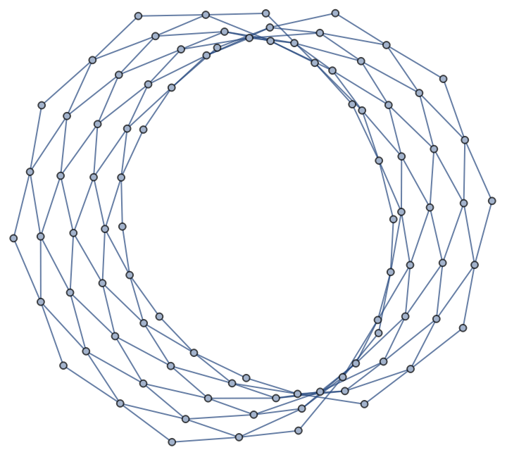
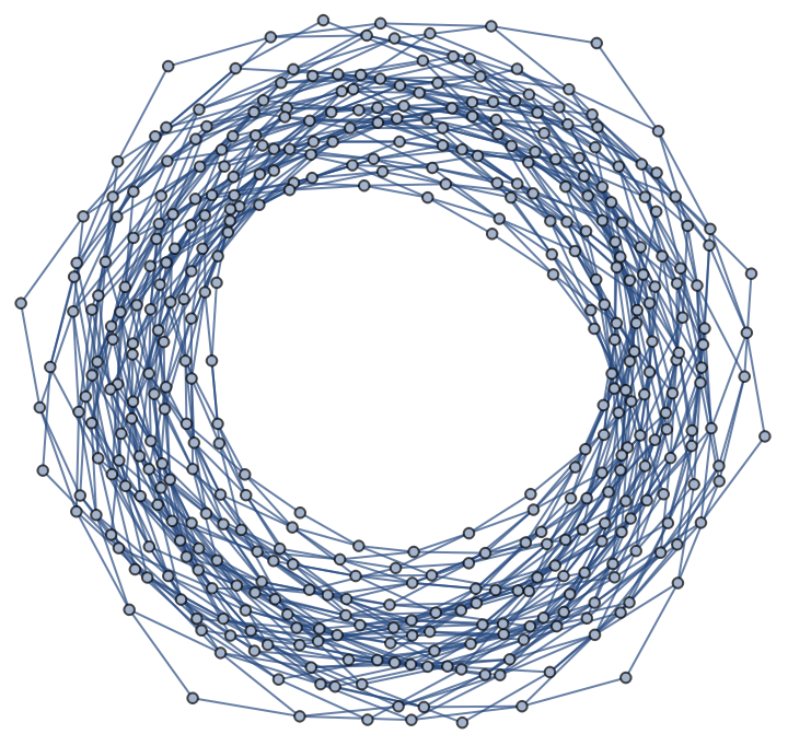
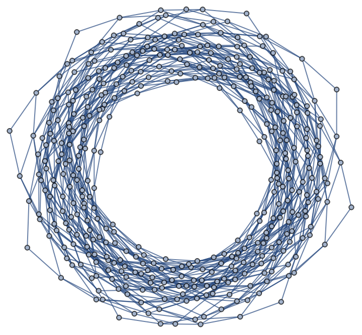
For example, for the N = 10 spins chain, the graph has the following form:
In[]:=
transitionGraph[10,#]&/@possibleSpinCycleEnergies[10]
Out[]=
,

,
,
,
,
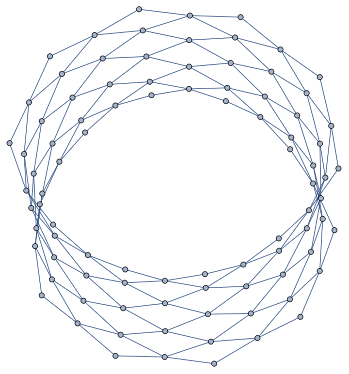

Note, the case corresponding to all pluses {+,+,...,+,+} corresponding to E = 10, and all flipping {+,-,+,-,...,-,+} corresponding to E = -10, has only two vertices.
As an example, the energies for the chains in a range from 1 to 10 are the following:
In[]:=
possibleSpinCycleEnergies/@Range[10]//Column
Out[]=
{1} |
{-2,2} |
{-1,3} |
{-4,0,4} |
{-3,1,5} |
{-6,-2,2,6} |
{-5,-1,3,7} |
{-8,-4,0,4,8} |
{-7,-3,1,5,9} |
{-10,-6,-2,2,6,10} |
Extension for the case of the 2D Ising model
Extension for the case of the 2D Ising model
Now we consider an extension for the case of 2D Ising model.
For the 2D case, we count over i and j (rows and columns). For illustration, take this configuration:
In[]:=
Matrix2DIsing={{-1,1,1},{1,-1,1},{1,1,-1}}
Out[]=
{{-1,1,1},{1,-1,1},{1,1,-1}}
The N×N Ising spin configurations can be constructed from the 1D stripes. We count all possible combinations of energies for the 1D strip as:
In[]:=
PossibleCombinationsOfEnergies1D[N_]:=Tuples[possibleSpinCycleEnergies[N],N]
For the 2D case in the nearest neighbors approximation, we count all possible energies both over i and j direction.
In[]:=
AllPossibleEnergies2D[N_]:=Tuples[Tuples[possibleSpinCycleEnergies[N],N],2]
For example, for the N = 3 case, there are the following combinations of energies over the rows and columns.
In[]:=
AllPossibleEnergies2D[3]
Out[]=
{{{-1,-1,-1},{-1,-1,-1}},{{-1,-1,-1},{-1,-1,3}},{{-1,-1,-1},{-1,3,-1}},{{-1,-1,-1},{-1,3,3}},{{-1,-1,-1},{3,-1,-1}},{{-1,-1,-1},{3,-1,3}},{{-1,-1,-1},{3,3,-1}},{{-1,-1,-1},{3,3,3}},{{-1,-1,3},{-1,-1,-1}},{{-1,-1,3},{-1,-1,3}},{{-1,-1,3},{-1,3,-1}},{{-1,-1,3},{-1,3,3}},{{-1,-1,3},{3,-1,-1}},{{-1,-1,3},{3,-1,3}},{{-1,-1,3},{3,3,-1}},{{-1,-1,3},{3,3,3}},{{-1,3,-1},{-1,-1,-1}},{{-1,3,-1},{-1,-1,3}},{{-1,3,-1},{-1,3,-1}},{{-1,3,-1},{-1,3,3}},{{-1,3,-1},{3,-1,-1}},{{-1,3,-1},{3,-1,3}},{{-1,3,-1},{3,3,-1}},{{-1,3,-1},{3,3,3}},{{-1,3,3},{-1,-1,-1}},{{-1,3,3},{-1,-1,3}},{{-1,3,3},{-1,3,-1}},{{-1,3,3},{-1,3,3}},{{-1,3,3},{3,-1,-1}},{{-1,3,3},{3,-1,3}},{{-1,3,3},{3,3,-1}},{{-1,3,3},{3,3,3}},{{3,-1,-1},{-1,-1,-1}},{{3,-1,-1},{-1,-1,3}},{{3,-1,-1},{-1,3,-1}},{{3,-1,-1},{-1,3,3}},{{3,-1,-1},{3,-1,-1}},{{3,-1,-1},{3,-1,3}},{{3,-1,-1},{3,3,-1}},{{3,-1,-1},{3,3,3}},{{3,-1,3},{-1,-1,-1}},{{3,-1,3},{-1,-1,3}},{{3,-1,3},{-1,3,-1}},{{3,-1,3},{-1,3,3}},{{3,-1,3},{3,-1,-1}},{{3,-1,3},{3,-1,3}},{{3,-1,3},{3,3,-1}},{{3,-1,3},{3,3,3}},{{3,3,-1},{-1,-1,-1}},{{3,3,-1},{-1,-1,3}},{{3,3,-1},{-1,3,-1}},{{3,3,-1},{-1,3,3}},{{3,3,-1},{3,-1,-1}},{{3,3,-1},{3,-1,3}},{{3,3,-1},{3,3,-1}},{{3,3,-1},{3,3,3}},{{3,3,3},{-1,-1,-1}},{{3,3,3},{-1,-1,3}},{{3,3,3},{-1,3,-1}},{{3,3,3},{-1,3,3}},{{3,3,3},{3,-1,-1}},{{3,3,3},{3,-1,3}},{{3,3,3},{3,3,-1}},{{3,3,3},{3,3,3}}}
So the total number of possible energy configurations is a product of 1D cases 8*8.
Now we count the total energy, both over the rows and columns.
For example, for the N = 3 case, they are the following.
In case we know a total energy over rows and columns, it can be constructed in from the 1D stripes. We find the combinations of the sums over i and j which give the total energy.
The positions which satisfy the energy conditions are (for our example case).
The
For example, for the 3×3 case with the energy = 10, there are the following possible combinations.
Now we need to generate all matrices with the energies specified before over the rows. For example, for the N = 3 case and our example, it is the following.
For higher dimensions, it can be extended by plugging Do cycle N times rather than 3 times: Do[Do[Do[Do[ ...],{i,1,Length[EnergiesRow1]},{i,1,Length[EnergiesRow2]}...{i,1,Length[EnergiesRowN]}]
The last step is to check whether our given combination satisfies the energy condition over the columns. For our example, it is the following.
This procedure can be generalized to an arbitrary N. One obstacle which I don’t know yet how to overcome, is how to implement Do[Do[Do[Do[... N times. Probably by recursion, but I did not figure it out yet.
Cellular Automaton rules preserving energy
Cellular Automaton rules preserving energy
Now we find all rules of CellularAutomaton (CA) under which the spin flips lead to transformations conserving energy. The values of spin can be +1 or -1, to convert it to the form amenable to CellularAutomaton, we make a shift 2CellularAutomaton[x,(#+1)/2]-1.
For example, rule 12 is the following.
The resulting CAs are:
They can be graphically represented as:
The corresponding pairs of CAs are the following:
Time dynamics of the spin system
Time dynamics of the spin system
With the rules which we found, we implement the time dynamics of the spin system. As the number of spins grows, the graphs are becoming messy. So, first we show the N = 5 case as an example.
The evolution graph has a form:
Interestingly, at some stage, we run out of options, and branchial graph becomes empty.
For another input state, we repeat the procedure.
Numerical analysis
Numerical analysis
We consider in detail the N = 10 case starting from the energy = 6, as the cases -10 and 10 are trivial.
We take the first element in the list.
We take the first element in the list.
We observe that on the 7th step the branchial graph really simplifies. Something resembling Poincare recurring theorem [10,11] except that the state is not the initial one, see below.
Observe that none of the vertices are the initial state. Let’s explore what happens next.
Ups... looks like evolution has stopped?
OK, let’s explore what happens if we plug the other state with the same energy = 6.
OK, let’s explore what happens if we plug the other state with the same energy = 6.
Ups... Looks like evolution has stopped again...
Evolution has stopped.
Evolution stopped at 5th step.
Stopped at the fifth step.
Stopped at the fifth step.
Finite Ring and Glauber’s solution.
Finite Ring and Glauber’s solution.
Now we compare the Branchial graphs with the Glauber’s solution.
The expectation value of the spin relaxes to zero. We plugged -20 to 20, but the exact Glauber’s solution has summation from negative infinity to positive infinity.
We will see the flattening below using the Branchial graphs, until the evolution is stopped.
... evolution stopped.
We see that after the second step the spins smooth out resembling the Glauber’s dynamics.
Local energy and entropy
Local energy and entropy
Examining local entropy and energy properties can reveal global properties such as freezing of the sample as a whole, e.g. global feature [12]. With the graphs derived in the previous section, we study the local energies of the chunks, as well as local and global entropy.
We observe that local and global entropies behave differently. Also, the chunk of larger size seems to look like a Gaussian, but a chunk of a smaller size seems to be looking opposite to the global entropy.
Future work
Future work
This research just started, and in the future, and we will explore this topic in depth.
Acknowledgments
Acknowledgments
Y.B. deeply appreciates the opportunity to participate in WSS 2022 and the help and useful discussion with all the members of the Wolfram Team, who really opened him a new world.
References
References
◼
[1] E. Ising, Z. Physik 31, 253 (1925).
◼
[2] L. Onsager, Phys. Rev. 65, 117 (1944).
◼
[3] Glauber, Roy J. “Time-dependent statistics of the Ising model.” Journal of mathematical physics 4.2 (1963): 294-307.
◼
[4] See, for example: https://reference.wolfram.com/language/ref/BesselJ.html, or G. N. Watson, Bessel Functions (Cambridge University Press, Cambridge, England, 1958)
◼
[8] Wolfram, Stephen. “Statistical mechanics of cellular automata.” Reviews of modern physics 55.3 (1983): 601.
◼
[9] Duminil-Copin, Hugo, and Vincent Tassion. “A new proof of the sharpness of the phase transition for Bernoulli percolation and the Ising model.” Communications in Mathematical Physics 343.2 (2016): 725-745.
◼
[10] Poincaré, H. (1890). “Sur le problème des trois corps et les équations de la dynamique”. Acta Math. 13: 1–270.
◼
[11] Poincaré, Œuvres VII, 262–490 (theorem 1 section 8).
◼
[12] Das, Tamoghna, and Tsvi Tlusty. “Positional information as a universal predictor of freezing.” Europhysics Letters 138.5 (2022): 57001.